Week 7 State of charge estimation
Aim: Simulate the 3 test cases from harness dashboard and write a detailed report on the results.
The closed-loop harness dashboard of the Battery management system is shown below.
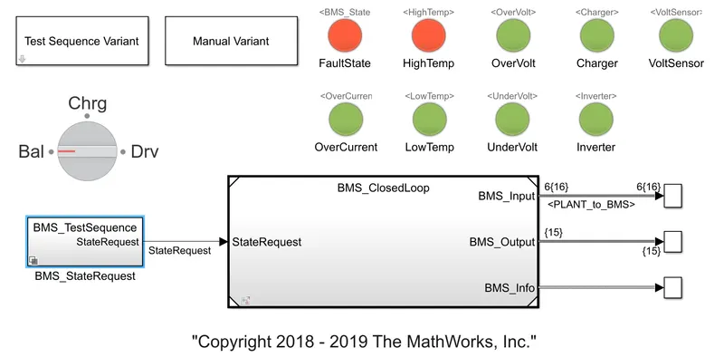
The above system model consists Test sequence variant through which we can implement the test cases. and BMS closed loop block and the results as the output.
A. Response of Test case 1:
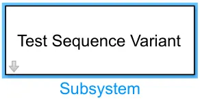
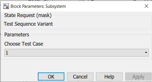
Goto the Test Sequence variant block shown above , and select the test case 1.
we can see the test case 1 details in the BMS state request block , which is input to the BMS Closed loop block.
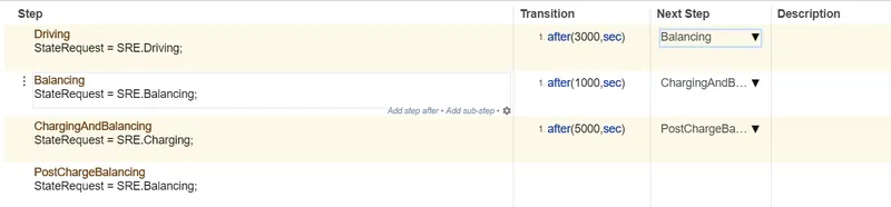
from above we can understand that driving is done for the first 3000 seconds , then after balancing is done for the 1000 seconds and then charging and also balancing is done for 5000 seconds, then after post charge balancing is done until the simulation is completed.
The scope results for the test case 1 are shown below:
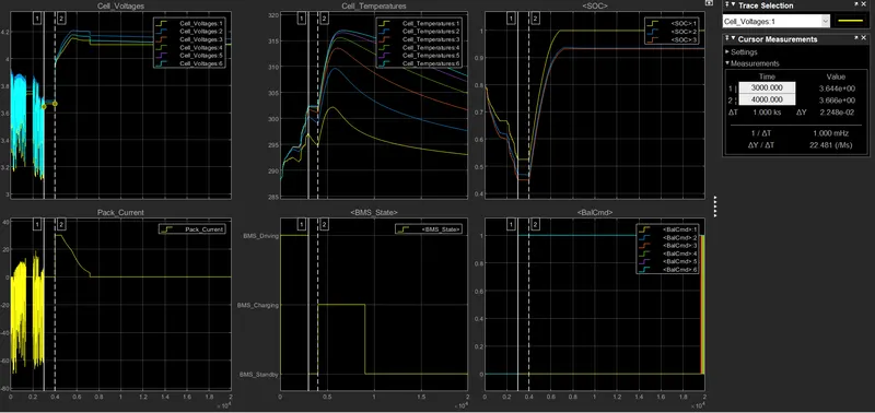
Observations:
1. The first plot on the left top corner shows us the responses of each 6 cell voltages with the time. The fluctuations in the cell voltages occur from 3.7volts to 3.2 volts, here the mode is driving mode so battery discharges , so the nominal voltage of the cell is 3.7volts and which is decreased to 3.2 volts. during the charging after driving mode , it reaches to 4.2 volts while charging the battery is in standby mode.
2. The whole battery pack current vs time is shown in the second plot(down). here we can see the negative direction of the current since the mode is driving mode reaches 60A in the negative direction.The current while charging it reaches 30A. and then fall down to zero Amp during the standby mode.
3. The battery packs cell temperature is shown in the 3rd plot on the top . it varies from the 290K and315K. the temperature of the cells increases up to 300k ,and then standbymode happens here the temperatures are decrease a bit by 2K each cell. and then charging occurs here each cell shows a sudden exponential peak and then exponentially falls down to 310k at fully charged position.
4.The Bms mode of state is shown in the bottom middle plot , here the modes at which time it happens are shown.For the first 3000seconds the driving mode is done. and the next 1000 seconds it is in standby mode and then charging mode for the 5000seconds and then standbymode till 20,000secods reached.
5. The Soc of the each cells are shown in the top right figure, here we can see the discharge and charging of the each cell , the soc of the cells is decreased to 40% , while in the driving mode, and then it is fully charged reached to 100% it maintains the full charge until the end of the simulation because of standbymode after full charge.
6. The cell balancing command signals are plotted in the bottom right figure.
B. Responce of the Testcase2:
The details of the test case 2 are:

here in the second test case we are giving 10,000seconds of driving mode and then charging for remaining 10,000 seconds.
The results of the Test case 2 are shown below:
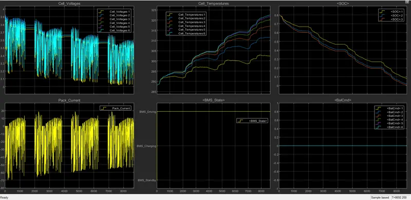
Observations:
* Here the current discharges in the driving mode upto 8700 seconds. so that means the a full charged battery diminishes after 8700 seconds, and here we used it continuously with out charging and standbymodes in the intermediate time.
* The voltages of each cells are ranged from 3.7 volts to 3 volts. Here we can understand that 3v are the cutoff voltage of each cell. the battery pack can discharge current upto 60A , can be considered as the maximum discharge current .The temperature of the cells increases in the driving mode and then continues to increase further because of the charging . The soc also decreases to zero percentage.
C) The Response of the Testcase 3:
The details of the 3rd test case are:

Now The battery pack is going to charge till 20,000 seconds.
The scope results for the Test case 3 are:
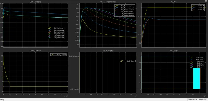
Observations:
*Since we are charging the battery pack through out the simulation time (20,000seconds), Intially the battery pack was charged to 80% and then reaches to 100%. After full charge The battery pack current increased to 30A and then drops to zero amperes . since there is nothing to charge the battery that is why the current drops to zero.
* The cell voltages reaches to approximately 4 to 4.2 volts stating it is the maximum charge voltage .During the charging the cell temperature increases once the charge completed the temperatures fall down and stabilizes.
-----------------------------------------------------------------
2. coloumb counting:
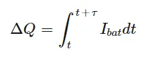
To estimate the SOC , we use the coloumb counting method by calculating the current .
we know that the charge can be found by integration of the current over time. so with in that time howmuch charge stored we can find.
The SOC of a battery pack can be estimated by voltage and current of the battery pack. we can find the battery operating mode whether discharging or charging by knowing the direction of the current .
The plant block model includes BMS ECU and PLANT is :
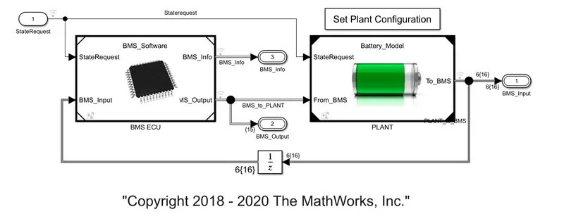
Here to estimate the SOC of the battery , we require information about the voltage and batterypack current.
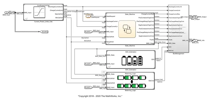
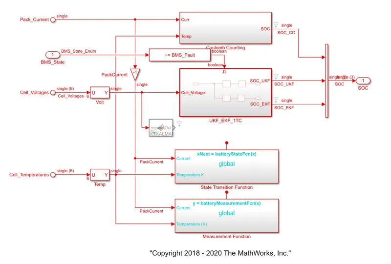
Here in the SOC estimate block three different estimations strategies for the SOC are shown. each style of estimation have advantages and disadvantages.
these are:1.coloumb counting
2.unscented approach
3. extended kalman filter approach
Here in coloumb counting block, there are two input signals one is current and other one is temperature,
current signal is multiplied by 1/3600 for converting seconds to hours ,and temperature is forwarded through current and time lookup table. both of these signals forwarded through split block, and the signal pushed to discrete-time integrator to trace the charge, so that we can estimate the state of charge of the battery pack.
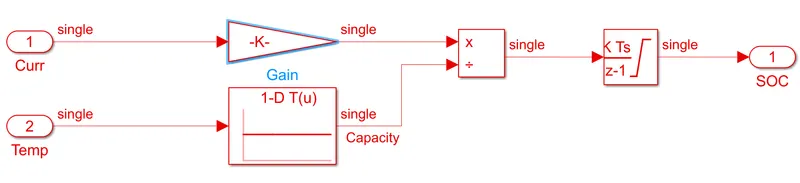
This method of estimation is very simple and low cost operational. but there is a chance of current sensing error.
* without the current flow we can not estimate the soc , it means we can not estimate a batteries initial SOC. this is a major drawback of this method of estimation.