Week 7 State of charge estimation
1.Simulate the 3 test cases from harness dashboard and write a detailed report on the results.
To simulate 3 test cases from the harness dashboard. We need to select the harness dashboard from the project file which we download with the reference link
The battery model harness dashboard overview is given below.
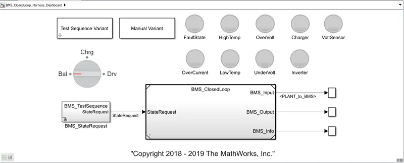
From the above MATLAB model we are Simulating 3 test cases from harness dashboard to find out the fault condition in BMS.
The dash board shows that where we can get the information related to the faults like over voltage, under voltage,high temperatue, over current and inverter related faults.
If there is any fault condition the indicators will turn to red colour otherwise it shows the green indication means there is no fault and the system is safe.
We can also know the information like the battery pack is in which condition at present moment like the mode of operation called Balancing mode, Charging mode and Discharging mode .
1. First test case from harness dashboard:
Select the Test sequence number one from the subsystem block.
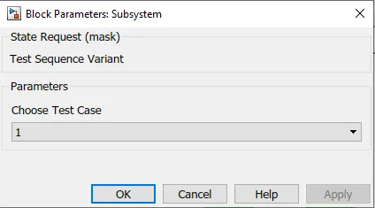
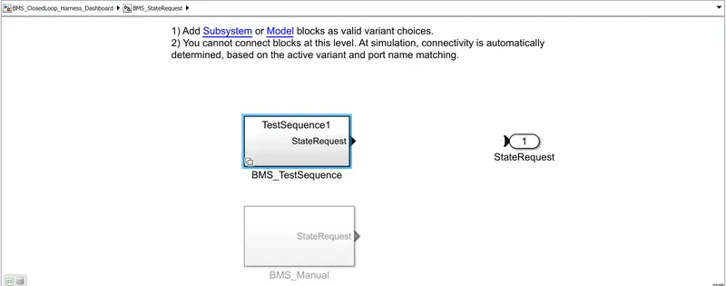
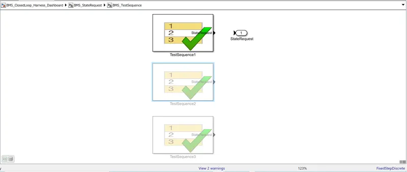
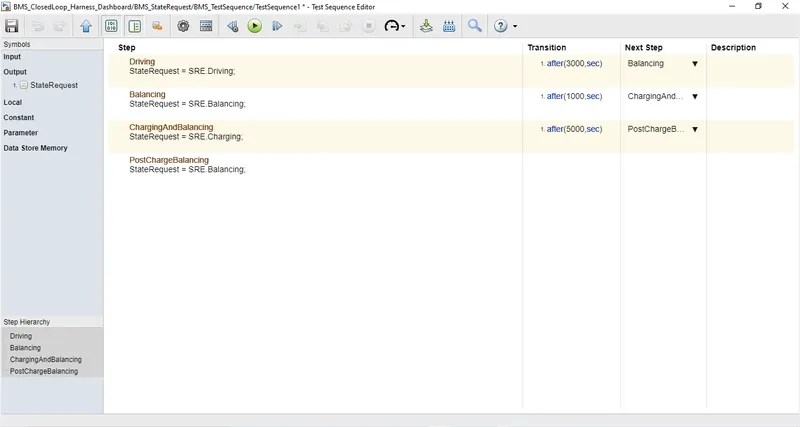
When simulation will start, the model will be in driving condition for 3000sec. After 3000 seconds it will be in balancing mode for 1000sec after 1000 sec it will be in charging and balancing mode for 5000sec. Now by running the simulation.
Output Results for first test:
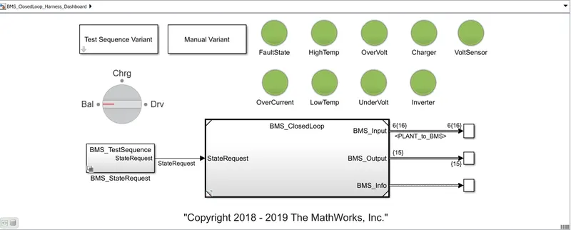
Here all the indicators are green. So we can see no errors and we check the plot for this model and is shown below.
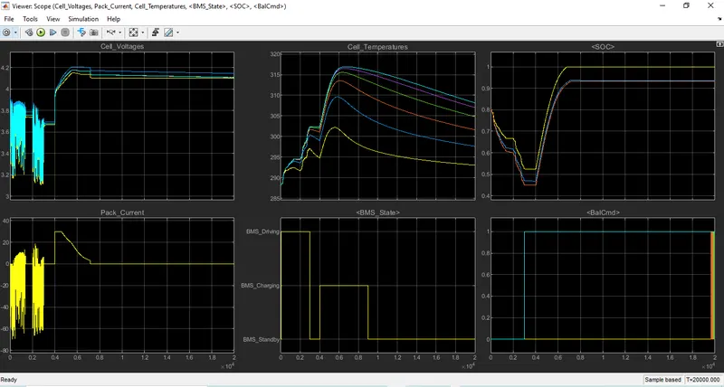
From the above plot, we can see the vehicle is initially in a driving state, and charging was done to 80%. After charging it reaches standby mode. It can be seen in the BMS state plot. Battery temperature increases in driving stage. The current plot shows the value of current supplied to the vehicle while driving. SOC decreased to 30% in driving conditions.
In charging stage SOC is initially is of 30% at this stage and increased to 100% or 1 to its full capacity and temprature also increases. Battery voltage was increased to 4.2V
2. Second test case from harness dashboard:
Now change the test sequence number to two from the subsystem block.
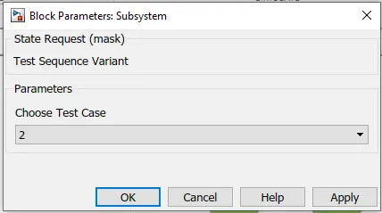
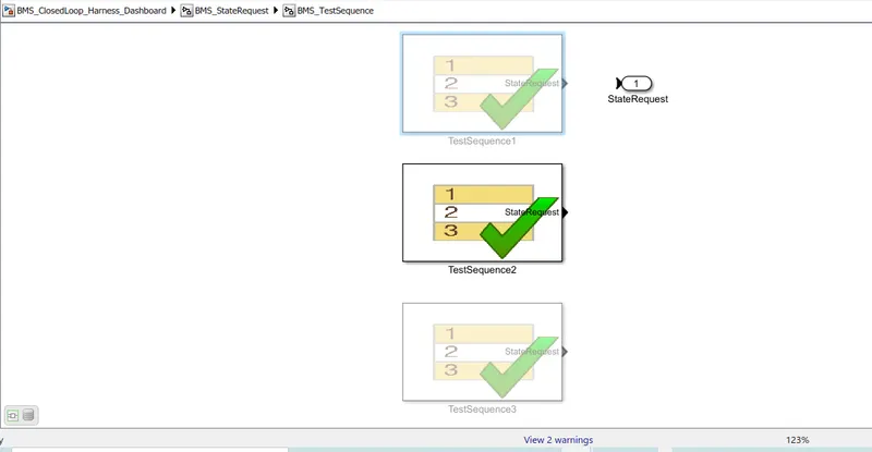
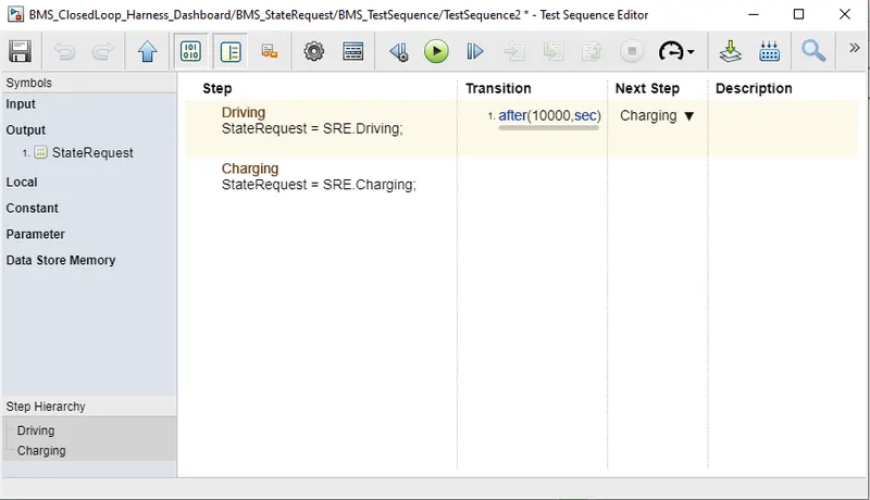
Here are the details of the test that will be performed in the simulation. The driving stage is from 0 to 10000 seconds and then charging.
Output Results for second test:
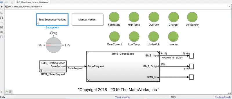
Here all the indicators are green. So we can see no errors and we check the plot for this model and is shown below.
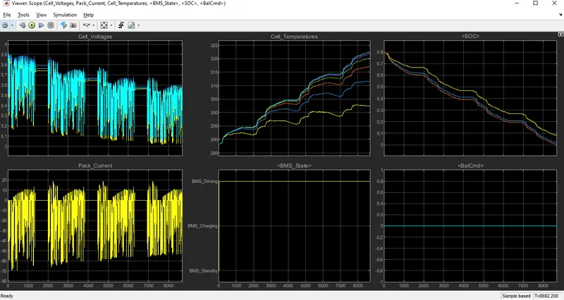
From the above plot we can observe.
Cell voltages reduced from initial 3.8V
Pack current reduced to 0
SOC is initially at 80% and reduced to 0%
Cell temperatures increased from initial 288.1k to a maximum recorded as 325k.
Cell Balancing is idle in this time period.
3. Third test case from harness dashboard:
Now change the test sequence number to three from the subsystem block.
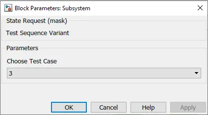
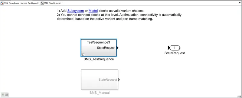
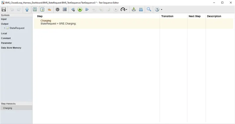
This test sequence had only one phase that is the charging phase for complete 20000 seconds.
Output Results for third test:
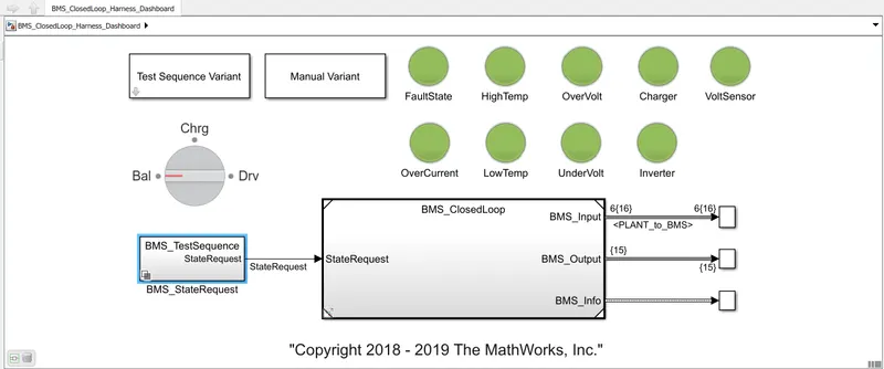
Here all the indicators are green. So we can see no errors and we check the plot for this model and is shown below.
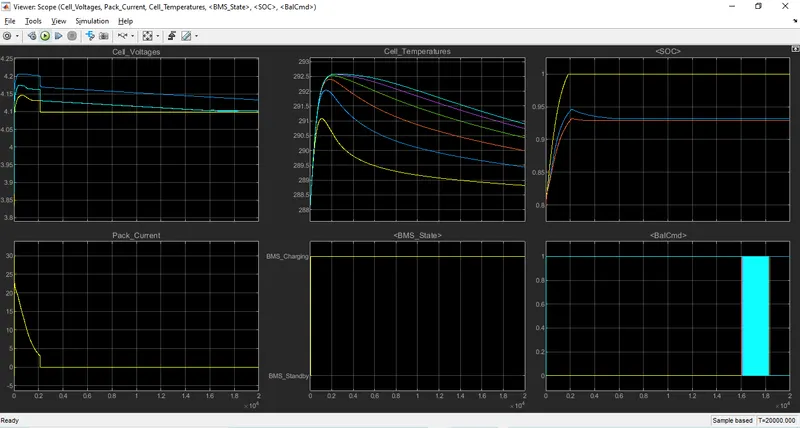
From the above plot we can observe.
The constant current (CC) and constant voltage (CV) characteristics of a battery pack.
From Initially time period of 0 sec the cell current increased to 30A and the cell voltages also gradually reached to 4.2V this phase of operation is called constant current or CC Mode.
At time instant of 0.2sec the cell voltages are gradually becomes constant till the end of the full charging voltage capacity of battery pack and at this time instant the current is gradually reduced to 0. So, this mode of operation is called constant voltage or CV Mode of operation.
SOC is initially is of 80% at time instant of 0.2 sec this is increased to 100%.
Cell temperatures increased from initial 288 to a maximum recoded as 292.5.
Cell Balancing is operating in this time period to ensure the maximum capacity reached by all the cells while charging in equal mode of operation and at time period of 1.8 sec the cell balancing is cutoff.
2 . What is coulomb counting? Refer to the above model and explain how BMS implements coulomb counting for SOC estimation?
Coulomb counting:
The Coulomb counting method measures the discharging current of a battery and integrates the discharging current over time in order to estimate SOC.
Coulomb counting method is done to estimate the, which is estimated from the discharging current, and previously estimated SOC values. SOC is calculated by the following equation:
SCO(t) = SOC(t − 1) +( I(t)/Qn)*Δt
But there are several factors that affect the accuracy of the Colomb counting method including temperature, battery history, discharge current, and cycle life.
Modified Coulomb Counting Method:
To improve the Coulomb counting method, a new technique called the modified Coulomb counting method is proposed. The modified Coulomb counting method uses the corrected current to improve the accuracy of estimation.
The corrected current is the function of discharging current. There is a quadratic relationship between the corrected current and discharging current of the battery. By the practice of experimental data, the corrected current is calculated by the following form:
Ic(t) = K1 I(t)2 + K2 I(t)+ K0
where K1 , K2 and K0 are constant values obtained from the practice experimental data.
Now we can see it in the project file we downloaded. A BMS system is the file represented below.
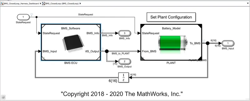
Click on the BMS ECU we get the Subsystem
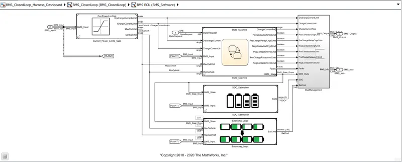
By clicking on the SOC estimation block we get the coulomb counting subsystem.
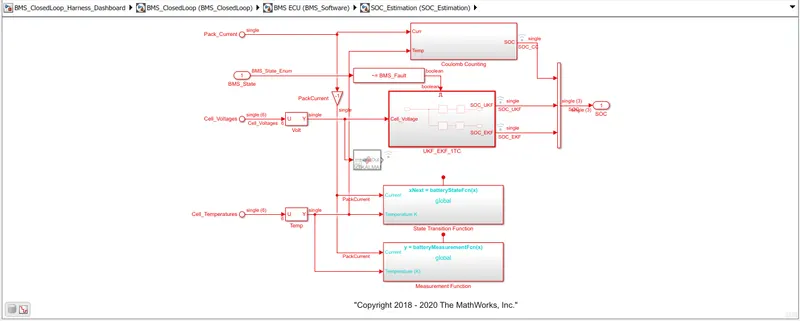
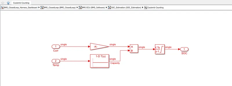
The above represented system only does the estimation by coulomb counting equation mentioned above.
Advantage of coulomb counting method is its simplicity and low computational cost.
Temperature and current from the battery is given as inputs.
Current signal is given to a gain block and temperature is given to capacity since it varies according to temperature.
These inputs are given for integration where current will be integrated with respect to time.
This outout is given to another block where it is divided by capacity.
Hence the SOC is estimated.