Week 7 State of charge estimation

1.

Initially as given we have to simulate 3 test cases from harness dashboard of the given model.This Model represents how the BMS reacts and gives information of any fault occuring in the battery pack with the help of lamos indicating what sort of fault is occured to the pack. The battery model harness dash board is represented below.

Matlab Model of harness dashboard:

 

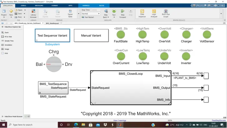
According to the question the test cases can be changed in the Test Sequence variant by selecting the required case as shown

  

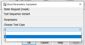
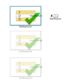
CASE 1:

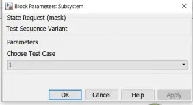
By changing the test case to 1 we can run the simulation of case 1 of harness dashboard.

 

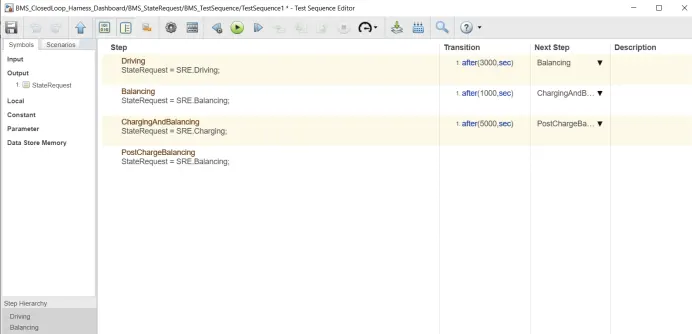
From the above fig we can observe that, when simulation will start, the model will be in driving condition. After 3000 seconds it will be in standby mode and after 1000 seconds it will be in charging mode. And after running the simulaiton we observe the results.

RESULTS 1:

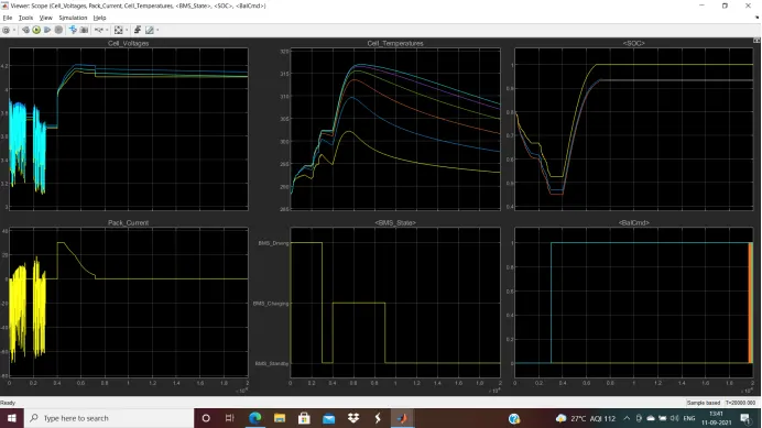
• From the plot we can see in the BMS state plotthat the vehicle is initially in driving state and then charging was done till 90%. After charging it reaches to standby mode.
• At the beginning of the simulation, the voltages are slightly different and are deflecting between 1 V to 3.9 V for 3000sec. And then all the  cells attain balance state such that there is a sudden rise in cell voltage till they reach 4.1 to 4.2 V at that instance the system goes on standby mode.
• The current graph is in the same manner but in the opposite direction when voltage is getting drop current required is high and current flows in the range of -70 A to 20 A.
• The temperature starting from the range of 289-degree Celcius and they get scattered to different temperatures of all cells. The cell temperature increases in driving stage as vehicle is in driving mode then during balancing stage , cell temperature reduces and then at start of charging the temperature increases suddenly then latter at charging and post charge balancing , the cell temperature shows the reducing behaviour.
• The soc of three different battery cell eachis performed with different matter yellow corresponds to column counting, blue corresponds to ukf and orange to ekf. During driving state , the SOC reduces from 80% to 45% during balancing state, SOC remains constant at 45% during charging stage , the SOC increases to 100 % and then remains constant.

CASE 2:

By changing the test case to 2 we can run the simulation of case 2 of harness dashboard.

 

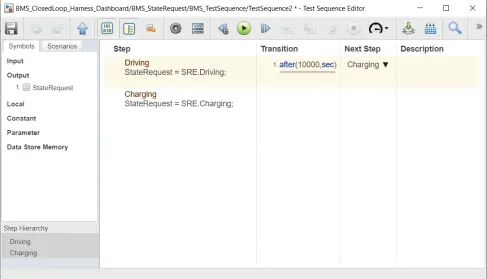
From the above fig we can observe that, when simulation will start, the model will be in driving condition for 10000sec and then charging stage occurs.

RESULTS 2:

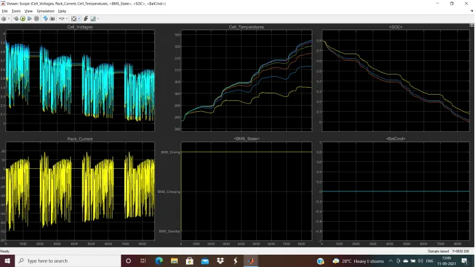
• From the plot we can see in the BMS state plotthat the vehicle is initially in driving state for 10000sec and then charging stage occurs.
• At the beginning of the simulation, the voltages are slightly different and are deflecting between 1 V to 3.9 V for 8500sec
• The current graph is in the same manner but in the opposite direction when voltage is getting drop current required is high and current flows in the range of -70 A to 20 A.
• The cell temperature increases as there is driving stage from 0 to 10000 second
• The SOC reducesfrom 80% to 0% and  then SOC do not increase beacuse there is no charging stage. And we can also observe that battery completly discharges at 9000 seconds so vehicle runs till 9000 seconds only.

CASE 3:

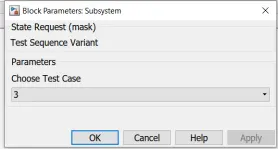
By changing the test case to 3 we can run the simulation of case 3 of harness dashboard.

 

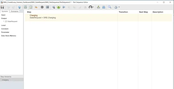
From the above fig we can observe that, when simulation will start, the model will be in charging condition for 20000sec.

RESULTS 3:

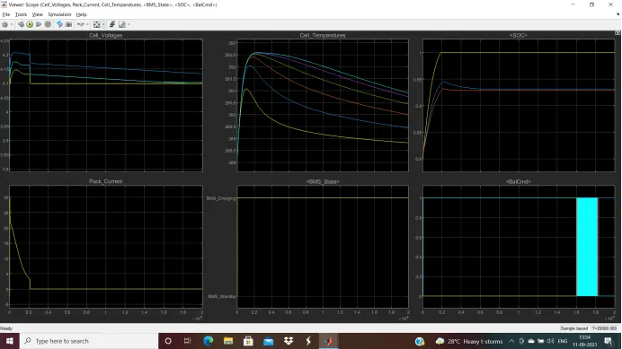
• From the plot we can see in the BMS state plotthat the vehicle is in charging state for 20000sec.
• In voltage plot ,the voltage increased upto a value of 4.2 V and then it gain a steady state of around 4.15V.
• the battery pack current is initiated with 20 A and then it falls to zero current till its complete simulation time of 0.2*10^4 sec and then it maintains the constant current because it is put on charging state and it remains constant throughout the simulation.
• Initially SOC was 80% but after 2000sec it reaches 100% as the mode here is charging mode for throughout the simulation.

2.

Coulomb Counting Method: 

The Coulomb counting method measures the discharging current of a battery and integrates the discharging current over time to estimate SOC. Coulomb counting method is done to estimate the SOC(t), which is estimated from the discharging current, I(t), and previously estimated SOC values, SOC(t-1). SOC is calculated by the following equation:

 

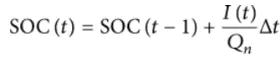
But several factors affect the accuracy of the Coulomb counting method including temperature, battery history, discharge current, and cycle life.

Modified Coulomb Counting Method:

To improve the Coulomb counting method, a new technique called the modified Coulomb counting method is proposed. The modified Coulomb counting method uses the corrected current to improve the accuracy of estimation. The corrected current is the function of discharging current. There is a quadratic relationship between the corrected current and discharging current of the battery. By the practice of experimental data, the corrected current is calculated by the following form

 

where K1, K2, and K0 are constant values obtained from the practice experimental data. In the modified Coulomb counting method, SOC is calculated by the following equation:

 

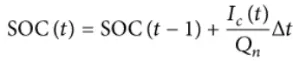
The experimental results show that the accuracy of the modified Coulomb counting method is superior to the conventional Coulomb counting method.

Coulomb counting for SOC estimation in given model:

 

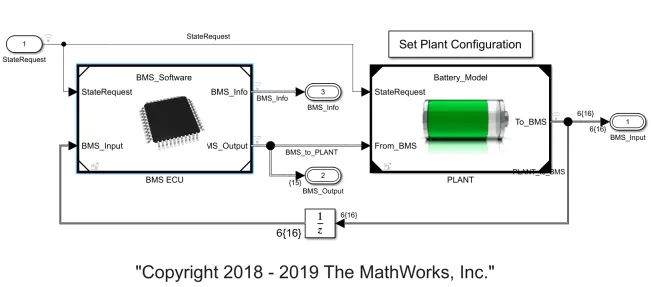
Given model contains BMS ECU and PLANT blocks. In this we observe how the coulomb counting is implementing in the BMS ECU block.

 

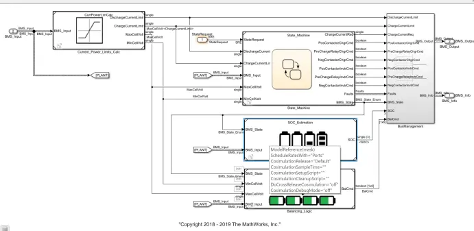
After opening th eBMS ECU block we can observe the State machine machine, SOC estimation and Balancing logic blocks out of which we need to click the SOC estimation block to get the coulomb counting.

 

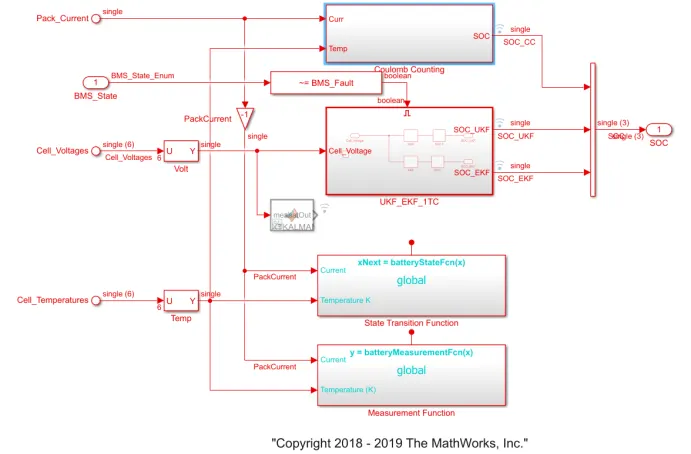
In the SOC estimation block we can see three different techniques for the state of charge estimation out of which the first method is columb counting and the other two are unscented(ukf) and extended Kalman filter(ekf). Here to open the couloum counting block to know the process.

 

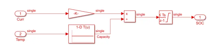
From the coulomb counting block we can observe in this method that the two input signals current and temperature are taken the curent signal goes to gain block and the temperature signal goes to current look up table. then as seen , signals are multiplied and divided as shown and then output is given to discrete time integrator to track the safe chargable time and then SOC is estimated.