Project

Aim: To study the system level simulation of All-Terrain Vehicle using Simulink.

Objectives: To prepare a report og BAJA ATV with different models.

Introduction:

All-Terrain Vehicle:

An all-terrain vehicle is also known as a light utility vehicle. It is a vehicle that travels on low-pressure tires, with a seat that is straddled by the operator, along with handlebars for steering control. As the name implies, it is designed to handle a wider variety of terrain than most other vehicles.

Main Components:

Generic Engine:

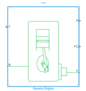
The Generic Engine block represents a general internal combustion engine. This block is a suitable generic engine for spark-ignition and diesel. Speed-power and speed-torque parameterizations are provided.
F and B are mechanical rotational conserving ports associated with engine crankshaft and block. While P and FC are physical signal output ports through which engine power and fuel consumption rate are reported.

Engine Sensor:

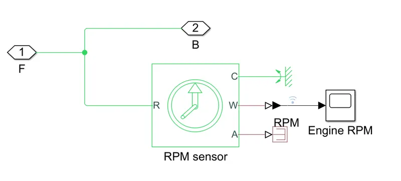
This block measures angular velocity. The sensor is ideal as it does not account for inertia, friction, delays, energy consumption.
The ports W and A reports the angular velocity and angular displacement respectively of port R relative to port C.

Simple gear:

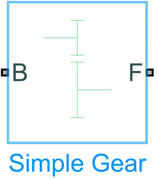
It is used in between the engine and the CVT block because to connect them it is need some speed reduction so simple gear block was used.
The port B is base gear and port F represents follower gear.

Continuously Variable Transmission(CVT):

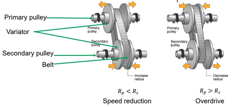
A CVT differ from traditional automatic transmissions in that they dont have gears that provide steps between low and high speed operatons. Instead they work with a pair of pulleys.
In CVT variable diameter pulleys plays a major role. In the pair of pulleys, one pulley is known as Primary pulley or Drive pulley which is connected to Crankshaft of the engine. The second pulley is known as Secondary or Driven pulley because it is driven by the first pulley and this pulley transfers energy to the driveshaft.
The Variator decides the Lower speed and higher speed. The variators are connected to the pulleys and the motion of variators decides the speed. As shown in above fig if the variator of primary pulley moves away and variator of secondary pulley comes close then the radius of the secondary increases , thus there will be reduction in speed and vice versa for the over drive.

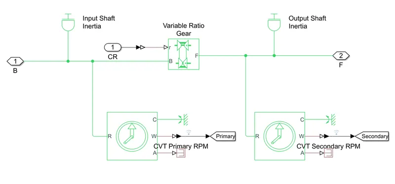
The above fig shows the CVT block. Port B is Drive pulley, F is Driven Pulley, r is Variable transmission ratio which is a input port. The input and output shaft inertia represents primary and secondary pulley respectively. The two rotational motion sensors are for tracking the angular velocities of the two pulleys.

Variable Transmission Ratio:

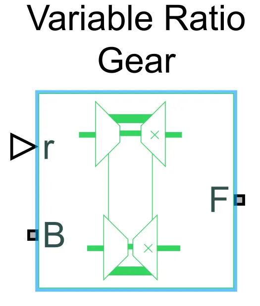
This block represents a variable ratio gearbox which is implemented by mechanical belt CVT.
This shows the variable transmission ratio block which consists port r which defines the ratio of input to output angular shaft velocities. Port B and F are mechanical rotational conversing ports.

Vehicle Body:

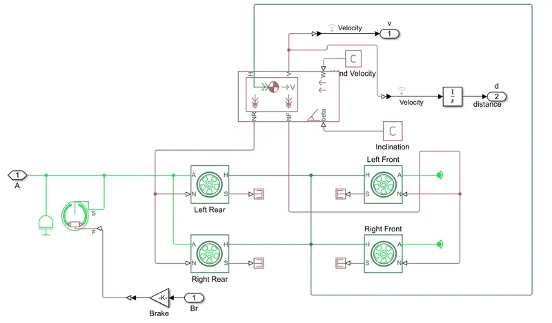
The vehicle body represents for body mass, aerodynamic drag, weight distribution between axles due to acceleration. The Double shoe brake is to apply brakes to the rear wheels.

Types of Models:

Model 1: BAJA ATV model without Dashboard

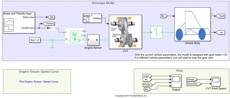
This model consists of signal builder, generic engine, motion sensors, CVT, vehicle body etc as shown.

Inputs:

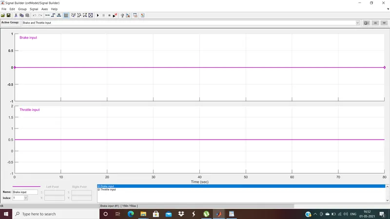
The signal builder is used as a input for brake, throttle and gear ratio. The brake input value is maintained as 0 and the throttle input is given as 0.5 for complete simulation as shown in above fig.

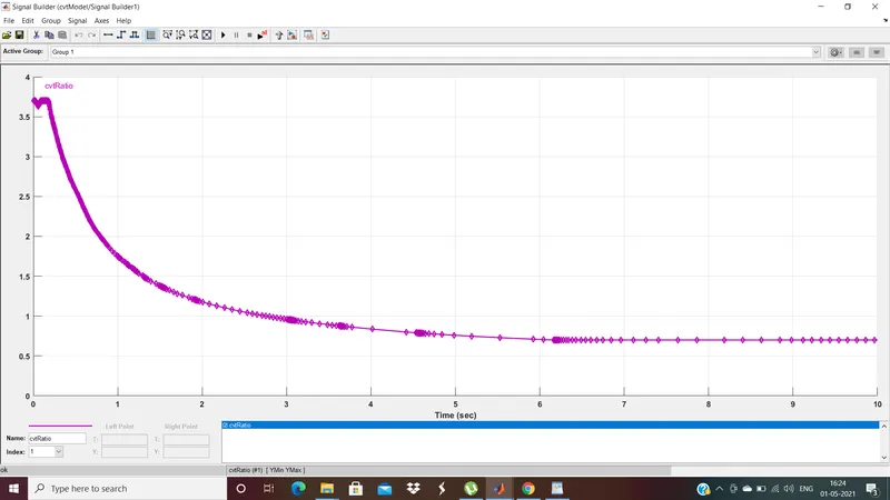
And this shows the cvt gear ratio input.

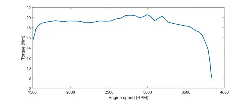
This is a Torque and speed curve, these are inputted from the workspace to generic engine block to generate output rpm and this is common for all the models in this report.

Results:

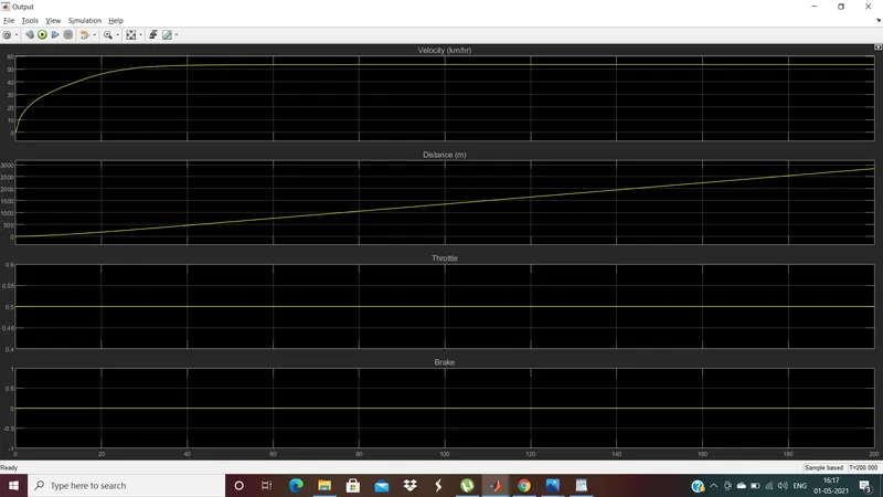
From this we can observe that there is a gradual rise in speed from rest position and remains constant after 30 sec as the throttle is give constant for all the simulation. As brake is given 0, it has no effect on velocity.

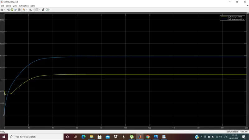
These graphs shows the variation in angular velocities of input and output shafts of varaible transmission system. These values differ with respect to the gear ratio. Initially CVT gear ratio input is above 1 so the secondary rpm is lower than the primary because the output shaft rotates slower to provide more torque and after few seconds the input is below below 1 then the secondary became higher than the primary rpm as the velocity of vehicle increases with reduction in torque.

Model 2: BAJA ATV model with Dashboard

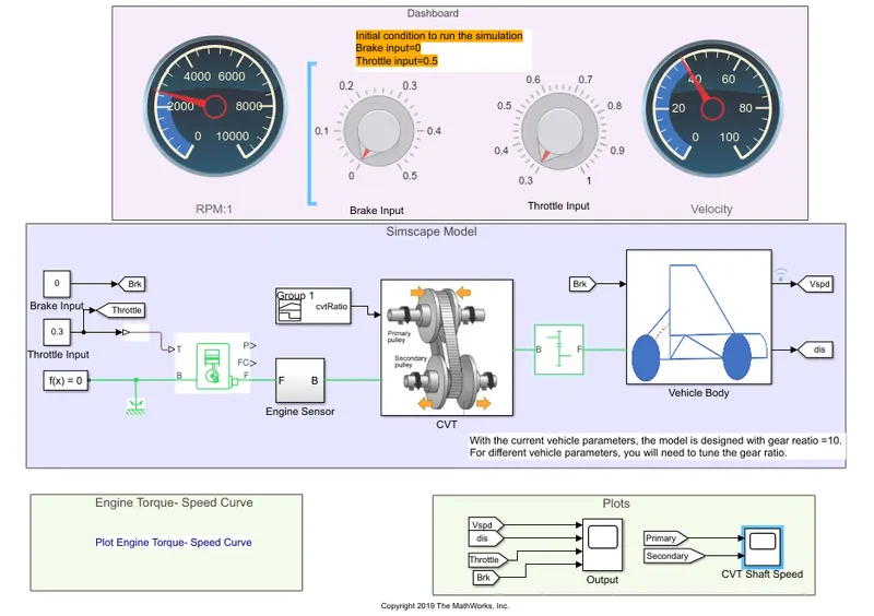
This model represents the BAJA ATV model with a dashboard. the only difference between model 1 and 2 is that the throttle and breake inputs are given by a dashbord control knob blocks during the simulation is running for infinite time period, so that the inputs are not constant like in model 1 and can be varied during simulation.

Results:

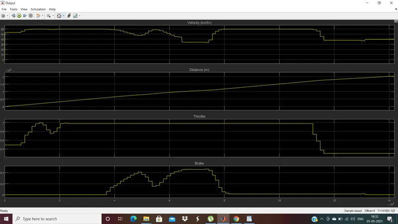
Here the engine speed is generated according to the inputs like throttle, break which are controlled by the user. From the graph we can observe that initially the throttle value is 0.5 and brake is 0 so the velocity increases from 0 to 55kmph. And the velocity is varied according to the variations in throttle and brake i.e., velocity decreased when brake increased and vice versa. This explains the direct relation of velocity w.r.t. throttle and brake inputs.

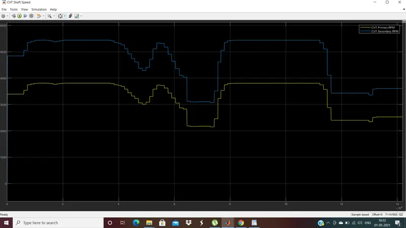
These graphs shows the variation in angular velocities of input and output shafts of varaible transmission system. These values differ with respect to the gear ratio.

Model 3: BAJA ATV model using Lookup table

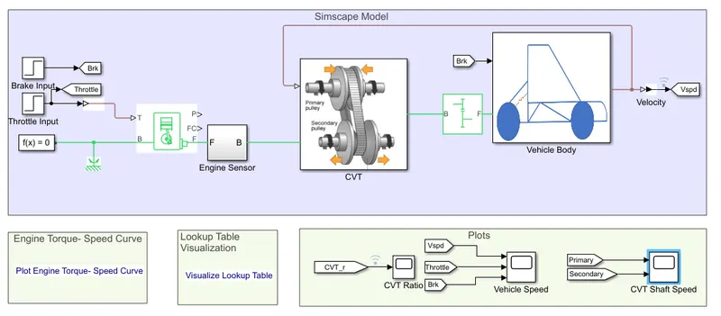
This model represents the BAJA ATV model using a lookup table. The only difference of this modek with the model 1 was that in this model the gear ratio input to CVT is provided by a lookup table and the remaining are same as before. The vehicle speed is given as feedback to CVT ratio lookup table.

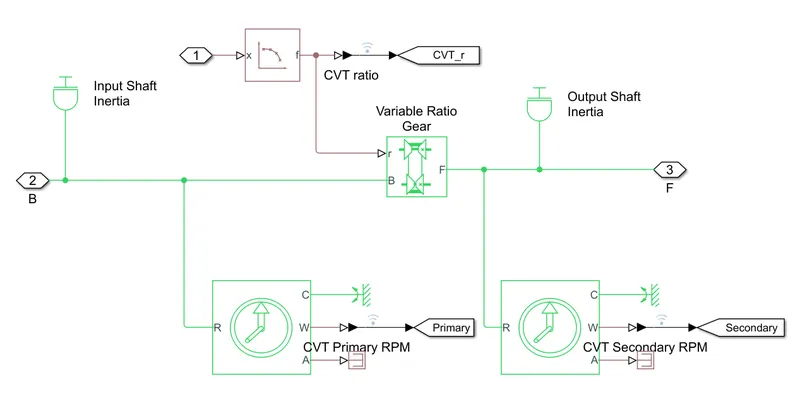
From the CVT block we can observe the lookup table connected to Variable gear ratio.

Inputs:

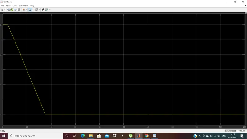
This is the plot of CVT gear ratio.

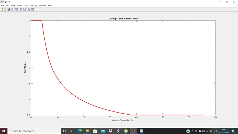
From this Lookup table visualization we can observe that velocity changes w.r.t. CVT ratio. Thus vehicles accelerates and decelerates when CVT ratio varied.

Results:

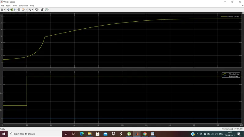
Here throttle is given 0.3 for 20 sec and after that increased to 1 while brake is given 0 and has no effect on velocity. Initially velocity is zero and gradually increasing and when after 20sec as throttle value increased the velocity aslo drastically increased.

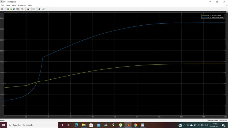
From the CVT ratio input we can observe that the input is above 1 for about 30 sec, till the primary rpm in CVT is higher than the secondary. After 30 sec the input value is below 1 and then the secondary rpm rised and it is higher than the primary rpm.
Initially the primary rpm is higher than secondary due to high torque requirement to change vehicle from rest to motion. then secondary rpm increases as the torque reduces when vehicle comes to motion.

Model 4: BAJA ATV model using Lookup table with Dashboard

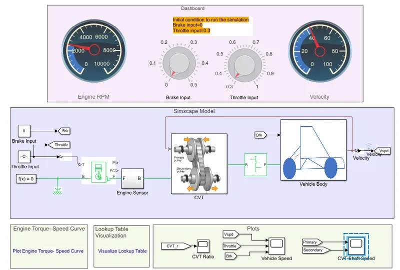
This model represents the BAJA ATV model using a lookup table with a dashboard. The only difference of this modek with the model 3 was that in this model dashboard is used for throttle, brake inputs and the remaining are same as before.

Results:

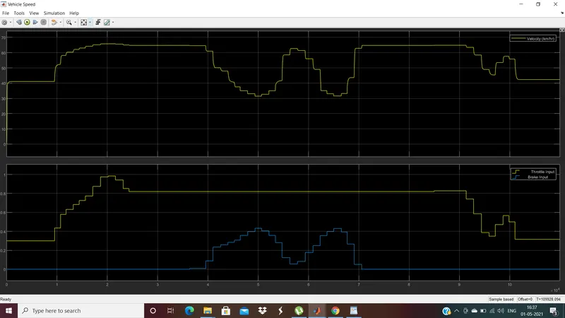
Here the engine speed is generated according to the inputs like throttle, break which are controlled by the user. From the graph we can observe that the velocity is varied according to the variations in throttle and brake i.e., velocity decreased when brake increased and vice versa. This explains the direct relation of velocity w.r.t. throttle and brake inputs.

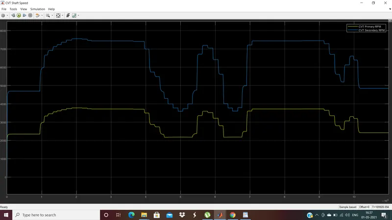
These graphs shows the variation in angular velocities of input and output shafts of varaible transmission system. These values differ with respect to the gear ratio which taken as a feedback from the vehicle speed which changes w.r.t. to dashboard inputs.

Conclusion:
Thus the 4 different models of BAJA ATV with CVT are analysed and observed the effect of CVT on vehicle velocity with multiple situations with respect to variation in throttle and brake inputs.