Week 7 - Simulation of a 1D Supersonic nozzle flow simulation using Macormack Method

AIM:To solve 1D Supersonic nozzle flow simulation using Macormack Method

• To simulate the isentropic flow through a Quasi 1D subsonic-supersonic nozzle.
• Derive both the conservation and non-conservation forms of the governing equations and solve them using MacCormack’s technique.
• To determine the steady-state temperature distribution for the flow-field variables and investigate the difference between the two forms of governing equations by comparing their solutions.
• To show the following plots inside the report
  • Steady-state distribution of primitive variables.
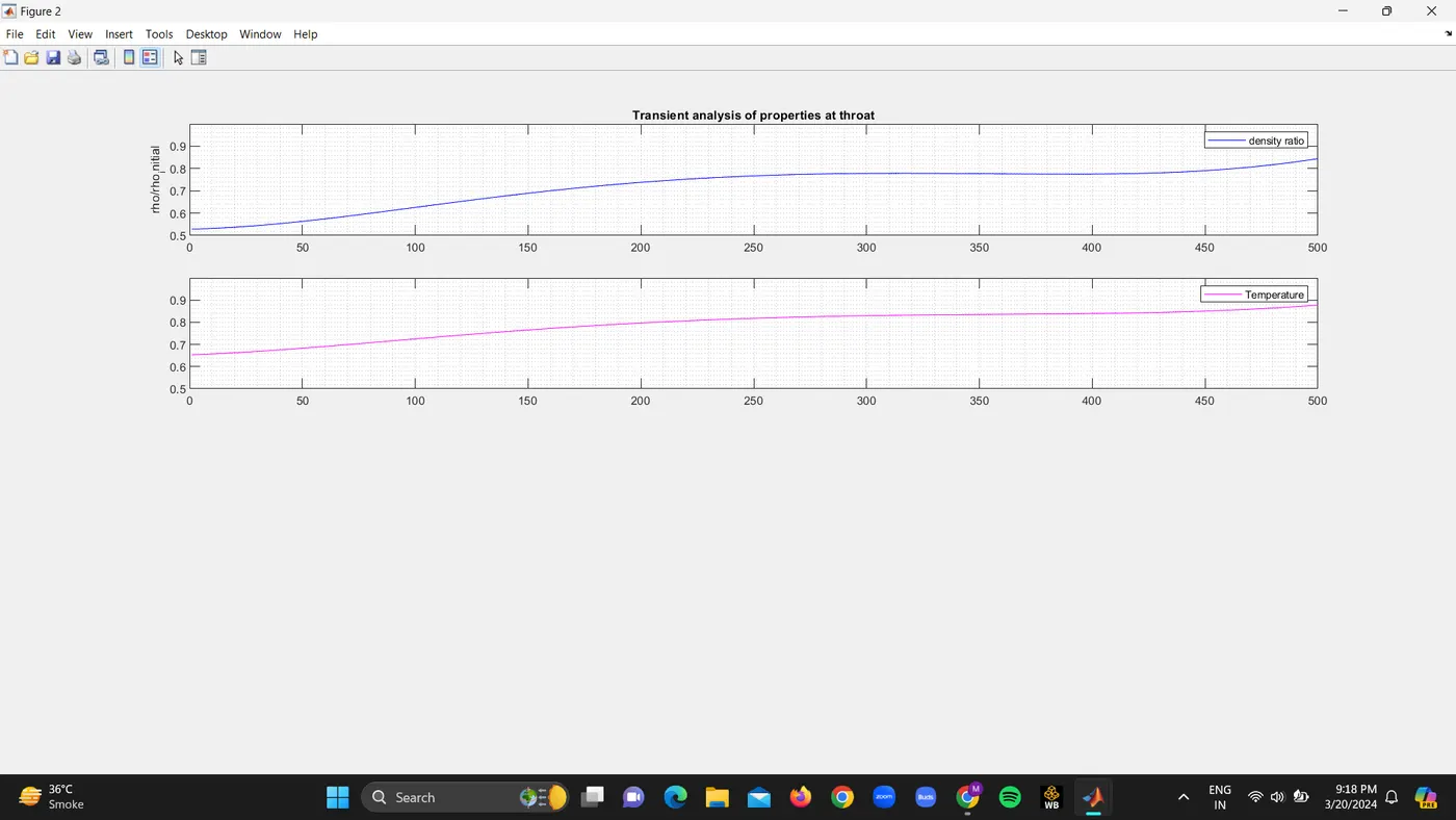
  • Time-wise variation of primitive variables.
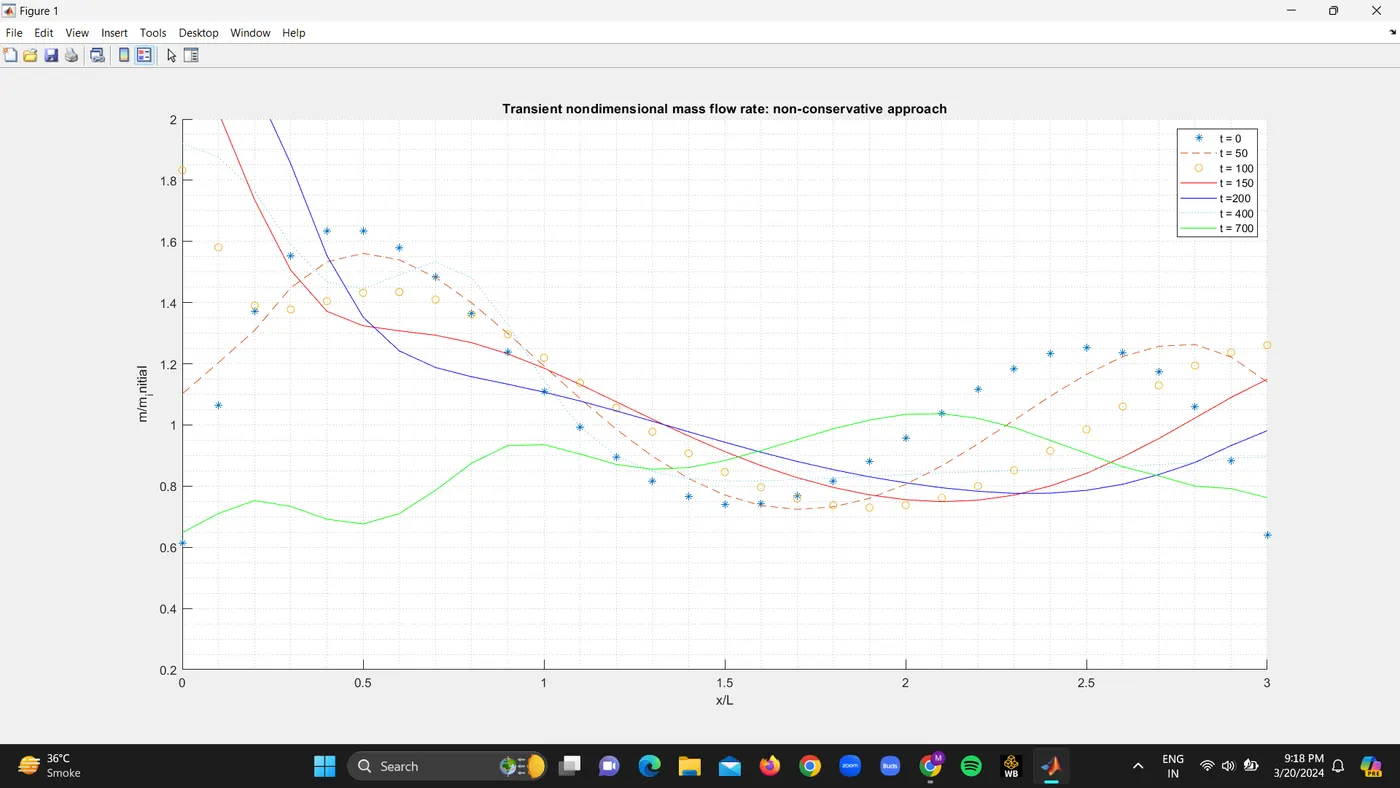
  • Variation of mass flow rate distribution inside the nozzle at different time steps during the time-marching process.
  • Comparison of normalized mass flow rate distributions of both forms.

Highlights:

• Perform a grid independence test on the solution and explain all your findings.
• The code must be modular. Write separate functions to solve both forms.
• Discuss all the plots that will be provided with observed inferences.

Procedure:

Considerations

• Consider a steady, isentropic flow through the converging-divergent nozzle as shown in the figure above.
• The flow at the inlet of the nozzle comes from a reservoir where pressure and temperature are denoted by Po and To. These are stagnation values.
• At the throat, sonic values of pressure and temperature are denoted by P* and T*, respectively.
• The area at the sonic throat is denoted as A*.
• In the subsonic inlet, it is assumed that the cross-sectional area of the reservoir is large, so the velocity is considered very small.
• In the divergent nozzle, the flow expands isentropically to supersonic speed at the exit.
• At the supersonic outlet, the exit pressure, temperature, velocity, and Mach number are denoted by Pe, Te, Ve, and Me. The force exerted on the gas to accelerate through the nozzle depends on the pressure ratio.
• Pressure ratio = PoPe">PoPe����

• It is assumed that the flow is a quasi-1D flow. This means that the flow properties will vary primarily along one direction, i.e., the x-direction only.

MacCormack Technique

It is an explicit finite difference technique that is second-order accurate in both space and time. The solution is obtained in three steps:

• Predictor Step

Forward differencing schemes are used for spatial derivatives and calculate the solution gradient, following which we obtain an intermediate solution (with initial conditions and calculated solution gradient)

• Corrector Step

Backward differencing schemes are used for spatial derivatives and calculate the solution gradient, following which we obtain a corrected solution (predicted values and solution gradient)

• Final Solution

The average for the two solution gradients (the predictor as well as corrector) is taken and from the initial state, the averaged solution gradient is added to obtain the final solution.

Setup

1. The governing equations are to be couched in terms of partial differential equations suitable for the time-marching solution of quasi-one-dimensional flow.
2. The finite-difference expressions pertaining to MacCormack’s technique as applied will be set up.
3. Other details for numerical solutions, such as the calculation of the time step and the treatment of boundary conditions, are to be formulated.

Conservation

Conservation form refers to an arrangement of an equation or system of equations, usually representing a hyperbolic system, which emphasizes that the property represented is conserved.

EULERIAN APPROACH →">→→ CONSERVATIVE FORM

The Eulerian approach refers to a fixed coordinate system in space and time, and the particles are studied with respect to this fixed system.

When the fundamental principles are derived using this approach, we get a conservative form.

Non-Conservation form

LAGRANGIAN APPROACH →">→→ NON-CONSERVATIVE FORM

In the Lagrangian approach, the fluid particles are followed as they travel through the flow. Fundamental principles derived from this approach, non-conservation forms of equations, are obtained.

Governing flow equations

• Non-dimensional variables

For nozzle flows, the flow field variables are frequently expressed in terms of nondimensional variables. The non-dimensional variables vary between 0 and 1, which is an aesthetic advantage when presenting the results.

Code:

% inputs
n= 31;
x = linspace(0,3,n);
dx = x(2)-x(1);
gamma = 1.4;
R = 287;

% calculate initial profiles
rho = 1-0.3146*x;
t = 1-0.2314*x;   % t = temperature
v = (0.1+1.09*x).*t.^0.5;

% area
a = 1+2.2*(x-1.5).^2;
n_throat = find((a-1)<0.001);

type_of_solver = input('select the type of solver: n=1 for non-coservative and n=2 for conservative');

% non coservative form solver

if type_of_solver == 1

    tic

    [rho,t,v,m,M,p_throat,rho_throat,v_throat,t_throat,M_throat,e] = non_conservative_nozzle(n,x,dx,gamma,a,R,n_throat);

    time_non_conservative = toc;

    fprintf('Computational Time: Non-Conservative Approach = %f sec',toc)
    fprintf('\n Number of Iterations required = %f', e);

% Transient properties at throat

figure(2)
% density ratio
subplot(4,1,1)
plot(rho_throat,'b')
title('Transient analysis of properties at throat')
legend('density ratio')
ylabel('rho/rho_initial')
axis([0 500 0.5 1])
grid minor
% temperature
subplot(4,1,2)
plot(t_throat,'m')
legend('Temperature')
axis([0 500 0.5 1])
grid minor
%pressure
subplot(p_throat,'g')
legend('Pressure')
ylabel('P/P_initial')
grid minor
% Mach number
subplot(4,1,4)
plot(m_throat,'r')
legend('Mach number')
ylabel('M/M_initial')
axis([0 500 0.5 1])
grid minor
xlabel('Number of Iterations')

% steady profiles

figure(3)
% density ratio
subplot(4,1,1)
plot(x,rho,'b')
title('steady state profiles of nozzle')
legend('density ratio')
ylabel('rho/rho_initial')
grid minor
% temperature
subplot(4,1,2)
plot(x,t,'m')
legend('Temperature')
ylabel('T/T_{o}')
grid minor
%pressure
subplot(4,1,3)
plot(x,p,'g')
legend('Pressure')
ylabel('P/P_initial')
axis([0 500 0.5 1])
grid minor
% Mach number
subplot(4,1,4)
plot(x,m,'r')
legend('Mach number')
ylabel('M/M_initial')
axis([0 500 0.5 1])
grid minor
xlabel('Space Domain')

% Conservative form solver

elseif type_of_solver == 2

    tic

    [rho_c,v_c,t_c,p_c,M_c,m_c,rho_throat_c,v_throat_c,t_throat_c,M_throat_c,p_throat_c] = conservative_nozzle(n,x,dx,a,gamma,n_throat,R);

    time_conservative = toc;
    fprintf('Computational Time: Conservative approach = %f sec', toc)

    % transient properties at throat

    figure(2)
    % density ratio
    subplot(4,1,1)
    plot(rho_throat_c,'b')
    title('Transient analysis of properties at throat')
    legend('density ratio')
    ylabel('rho/rho_initial')
    axis([0 500 0.5 1])
    grid minor
    % temperature
    subplot(4,1,2)
    plot(t_throat_c,'m')
    legend('Temperature')
    axis([0 500 0.5 1])
    grid minor
    %pressure
    subplot(p_throat_c,'g')
    legend('Pressure')
    ylabel('P/P_initial')
    axis([0 500 0.5 1])
    grid minor
    % Mach number
    subplot(4,1,4)
    plot(m_throat_c,'r')
    legend('Mach number')
    ylabel('M/M_initial')
    axis([0 500 0.5 1])
    grid minor
    xlabel('Number of Iterations')

    % steady profiles

    figure(3)
    % density ratio
    subplot(4,1,1)
    plot(x,rho_c,'b')
    title('steady state profiles of nozzle')
    legend('density ratio')
    ylabel('rho/rho_initial')
    grid minor
    % temperature
    subplot(4,1,2)
    plot(x,t_c,'m')
    legend('Temperature')
    ylabel('T/T_{o}')
    grid minor
    %pressure
    subplot(4,1,3)
    plot(x,p_c,'g')
    legend('Pressure')
    ylabel('P/P_initial')
    axis([0 500 0.5 1])
    grid minor
    % Mach number
    subplot(4,1,4)
    plot(x,m_c,'r')
    legend('Mach number')
    ylabel('M/M_initial')
    grid minor
    xlabel('Space Domain')

end

FUNCTION CODE

Non-conservative;

function [rho,t,v,m,M,p_throat,rho_throat,v_throat,t_throat,M_throat,e] = non_conservative_nozzle(n,x,dx,gamma,a,R,n_throat)

% Initial Profiles

% Density,Temperature,Velocity
rho = 1 - 0.3146*x;
t = 1 - 0.2314*x;   
v = (0.1 + 1.09*x).*t.^0.5;
m = rho.*a.*v;
s = sqrt(rho.*R.*t);
% courant number limiting value
C = 0.5;
nt = 500;

% error
error = 9e9;
tol = 1e-4;

e = 0

while error > tol

    e = e + 1;

    rho_old = rho;
    v_old = v;
    t_old = t;
    m_old = rho_old.*a.*v_old;
    s_old = sqrt(t_old.*R.*gamma);


    % time step
    dt = min(C*dx./(s_old + v_old));

    % Predictor method
    for j =2:n-1

        drhodx = (rho(j+1)-rho(j))/dx;
        dvdx = (v(j+1)-v(j))/dx;
        dtdx = (t(j+1)-t(j))/dx;
        dlogadx = (log(a(j+1))-log(a(j)))/dx;

        % continuty equation
        drhodt_p(j) = -rho(j)*dvdx - rho(j)*v(j)*dlogadx - v(j)*drhodx;

        % momentum equation
        dvdt_p(j) = -v(j)*dvdx - (1/gamma)*(dtdx +(t(j)/rho(j))*drhodx);

        % energy equation
        dtdt_p(j) = -v(j)*dtdx - (gamma-1)*t(j)*(dvdx + v(j)*dlogadx);

        % solution update
        rho(j) = rho(j) + drhodt_p(j)*dt;
        v(j) = v(j) + dvdt_p(j)*dt;
        t(j) = t(j) + dtdt_p(j)*dt;

    end

        % corrector method
      for j =2:n-1
        
        drhodx = (rho(j)-rho(j-1))/dx;
        dvdx = (v(j)-v(j-1))/dx;
        dtdx = (t(j)-t(j-1))/dx;
        dlogadx = (log(a(j))-log(a(j-1)))/dx;

        % continuty equation
        drhodt_c(j) = -rho(j)*dvdx - rho(j)*v(j)*dlogadx - v(j)*drhodx;

        % momentum equation
        dvdt_c(j) = -v(j)*dvdx - (1/gamma)*(dtdx +(t(j)/rho(j))*drhodx);

        % energy equation
        dtdt_c(j) = -v(j)*dtdx - (gamma-1)*t(j)*(dvdx + v(j)*dlogadx);

      end

      % compute the average time derivative 

      drhodt = 0.5*(drhodt_p + drhodt_c);
      dvdt = 0.5*(dvdt_p + dvdt_c);
      dtdt = 0.5*(dtdt_p + dtdt_c);

      % final solution update

      for i = 2:n-1
        rho(i) = rho_old(i) + drhodt(i)*dt;
        v(i) = v_old(i) + dvdt(i)*dt;
        t(i) = t_old(i) + dtdt(i)*dt;

      end

      % Boundary conditions
      % inlet
      v(1) = 2*v(2) - v(3);

      % outlet
      rho(n) = 2*rho(n-1) - rho(n-2);
      t(n) = 2*t(n-1) - t(n-2);
      v(n) = 2*v(n-1) - v(n-2);

      % Parameters

      % Mach number
      M = v./s;

      % Mass flow rate
      m = rho.*a.*v;

      % Pressure
      p = rho.*t;

      % throat values
       rho_throat(e) = rho(n_throat)
       t_throat(e) = t(n_throat);
       M_throat(e) = M(n_throat);
       v_throat(e) = v(n_throat);
       p_throat(e) = p(n_throat);


      % time-loop error criteria for convergence 
      % mass-flow is used as the com[aring criteria, when mass-flow becomes
      % constant, it can be said that solution has converged

      error = max(abs(m - m_old));

      % capturing change in mass-flow before steady state is reached 

      figure(1);
      hold on;

      if e == 1
          plot (x,m,'*');
      elseif e == 50
          plot(x,m,'--');
      elseif e == 100
          plot(x,m,'o');
      elseif e == 150
          plot(x,m,'r');
      elseif e == 200
          plot(x,m,'b');
      elseif e == 400
          plot(x,m,':');
      elseif e == 700
          plot(x,m,'g');
      end

end

title('Transient nondimensional mass flow rate: non-conservative approach')
xlabel('x/L')
ylabel('m/m_initial')
legend('t = 0','t = 50','t = 100','t = 150','t =200','t = 400','t = 700')
axis([0 x(n) 0.2 2]);
grid minor;

end

%Conservative

function [rho_c,v_c,t_c,p_c,M_c,m_c,rho_throat_c,v_throat_c,t_throat_c,M_throat_c,p_throat_c] = conservative_nozzle(n,x,dx,a,gamma,n_throat,R)

nt = 500;
C = 0.5;

% intial values

for i = 1: length(x)
    if x(i) >= 0 && x(i) < 0.5
        rho_c(i) = 1;
        t_c(i) = 1;
    elseif x(i) >= 0.5 && x(i) < 1.5
        rho_c(i) = 1 - 0.366*(x(i) - 0.5);
        t_c(i) = 1 - 0.167*(x(i) - 0.5);
    elseif x(i) >= 1.5 && x(i) <= 3
        rho_c(i) = 0.634 - 0.3879*(x(i) - 1.5);
        t_c(i) = 0.833 - 0.3507*(x(i) - 1.5);
    end
end

v_c = (0.59)./(rho_c.*a);
rho_old_c = rho_c;
v_old_c = v_c;
t_old_c = t_c;

% time marching solution

U1 = rho_c.*a;
U2 = rho_c.*a.*v_c;
U3 = rho_c.*a.*((t_c./gamma - 1)) + ((gamma/2).*v_c.^2);

% time loop 

for k = 1:nt

    U1_old = U1;
    U2_old = U2;
    U3_old = U3;

    % time step
    a_c = sqrt(gamma.*R.*t_c);
    % courant time step
    TS = C*dx./(a_c + v_c);
    dt = 0.001;

    % flux vectors
    F1 = U2;
    F2 = (U2.^2./U1) + ((gamma-1)/gamma)*(U3-(gamma*U2.^2)./(2.*U1));
    F3 = (gamma*U2.*U3./U1) - ((gamma*(gamma-1)/2)*(U2.^3./U1.^2));

    % predictor step

    for j = 2:n-1

        J(j) = (1/gamma).*rho_c(j).*t_c(j).*((a(j+1)-a(j))/dx);

        % continuity equation
        dU1dt_c_p(j) = -(F1(j+1)-F1(j))/dx;

        % momentum equation
        dU2dt_c_p(j) = (-(F2(j+1)-F2(j))/dx) + J(j);

        % energy equation
        dU3dt_c_p(j) = -(F3(j+1)-F3(j))/dx;

        % predictor step solution update

        U1(j) = U1(j) + (dU1dt_c_p(j)*dt);
        U2(j) = U2(j) + (dU2dt_c_p(j)*dt);
        U3(j) = U3(j) + (dU3dt_c_p(j)*dt);

    end

    % presicted value of properties (variables) of interest and flux

    rho_c = U1./a;
    v_c = U2./U1;
    t_c = (gamma-1)*((U3./U1)-((gamma/2)*(U2./U1).^2));
    p_c = rho_c.*t_c;
    F1 = U2;
    F2 = (U2.^2./U1) + (((gamma-1)/gamma)*(U3 - (((gamma/2)*U2.^2)./U1)));
    F3 = (gamma*U2.*U3./U1) - ((gamma*(gamma-1)/2)*(U2.^3./U1.^2));

    % corrector step

    for j = 2:n-1

        J(j) = (1/gamma).*rho_c(j).*t_c(j).*((a(j)-a(j-1))/dx);

        % continuity equation
        dU1dt_c_c(j) = -(F1(j)-F1(j-1))/dx;

        % momentum equation
        dU2dt_c_c(j) = (-(F2(j)-F2(j-1))/dx) + J(j);

        % energy equation
        dU3dt_c_c(j) = -(F3(j)-F3(j-1))/dx;
    end

    % average time derivative
    dU1dt_c_avg = 0.5*(dU1dt_c_p + dU1dt_c_c);
    dU2dt_c_avg = 0.5*(dU2dt_c_p + dU2dt_c_c);
    dU3dt_c_avg = 0.5*(dU3dt_c_p + dU3dt_c_c);


        % final solution update
        for i = 2:n-1

        U1(i) = U1_old(i) + (dU1dt_c_avg(i)*dt);
        U2(i) = U2_old(i) + (dU2dt_c_avg(i)*dt);
        U3(i) = U3_old(i) + (dU3dt_c_avg(i)*dt);

    end

    % boundary conditions
    % inlet
    rho_c(1) = 1;
    t_c(1) = 1;
    U1(1) = rho_c(1)*a(1);
    U2(1) = 2*U2(2)-U2(3);
    U3(1) = U1(1)*(t_c(1)/(gamma-1)+(gamma/2)*v_c(1).^2);

    % outlet
    U1(n) = 2*U1(n-1) - U1(n-2);
    U2(n) = 2*U2(n-1) - U2(n-2);
    U3(n) = 2*U3(n-1) - U3(n-2);

    % calculation of properties (variables) of interest

    rho_c = U1./a;
    v_c = U2./U1;
    t_c = (gamma-1)*(U3./U1-(gamma/2)*v_c.^2);
    p_c = rho_c.*t_c;

    % calculation of remaining important properties
    
    %mach number
    M_c = v_c./sqrt(t_c.*gamma.*R);
    % mass flow
    m_c = rho_c.*a.*v_c;

    % throat values

    rho_throat_c(k) = rho_c(n_throat);
    t_throat_c(k) = t_c(n_throat);
    M_throat_c(k) = M_c(n_throat);
    v_throat_c(k) = v_c(n_throat);
    p_throat_c(k) = p_c(n_throat);

    % capturing change in mass-flow before steady state is reached

    figure(1);
    hold on;

    if k == 1
        plot(x,m_c,'*');
    elseif k ==50
        plot(x,m_c,'--');
    elseif k == 100
        plot(x,m_c,'o');
    elseif k == 150
        plot(x,m_c,'r');
    elseif k == 200
        plot(x,m_c,'b');
    elseif k == 400
        plot(x,m_c,':');
    elseif k == 700
        plot(x,m_c,'g');
    end

    end

    title('Transient non-dimensional mass flow rate: conservative approach')
    xlabel('x/L');
    ylabel('m/m_initial')
    legend('t=0','t=50','t=100','t=150','t=200','t=400','t=700')
    axis([0 x(n) 0.2 2]);
    grid minor;

end

Plot: