Week 7 - Simulation of a 1D Supersonic nozzle flow simulation using Macormack Method
Objective:
To simulate isentropic flow within a Quasi 1D subsonic nozzle, the governing equations must be derived in both conservation and non-conservation versions. These equations are then solved using the MacCormack's approach, which is available in MATLAB.
Problem Identification:
Determine the temperature distribution for flow-field variables in a steady-state and investigate the difference between the two forms of governing equations. This investigation is carried out by comparing their solutions and producing the following plots:
- The steady-state distribution of primitive variables within the nozzle is shown.
- The time development of primordial variables is shown.
- During the time-marching operation, the mass rate distribution within the nozzle can be observed at various time steps.
- The normalized mass flow rate distributions from both equation forms are compared..
Theory:
Although an analytical solution exists for such issues, it is impractical to seek a numerical solution for isentropic flow via a quasi-1D subsonic-supersonic nozzle. Our goal, however, is not to replicate an approximate analytical answer. Rather, we want to show off the improved capabilities of Computational Fluid Dynamics (CFD) in a variety of fields. In this situation, both the Conservative and Non-Conservative forms are used to provide a numerical solution.
The Time Marching method is used to solve this problem by advancing the governing equations in terms of Partial Differential Equations (PDEs) for both forms. These forms are only expressed in numerical terms; upon closer inspection, all techniques are similar.
Upon observing these amplification factors, it's evident that the outcomes showcased in the graph fail to converge. Instead, errors progressively escalate to the extent that MATLAB eventually reaches its computational limits.
We concentrate on isentropic flow via a convergent-divergent nozzle. The flow comes from a reservoir at the nozzle's intake. The velocity is noticeably low due to the reservoir's relatively huge cross-sectional area. The flow stays locally subsonic during the nozzle's convergent length, changes to sonic conditions near the throat, and eventually reaches supersonic within the divergent region.
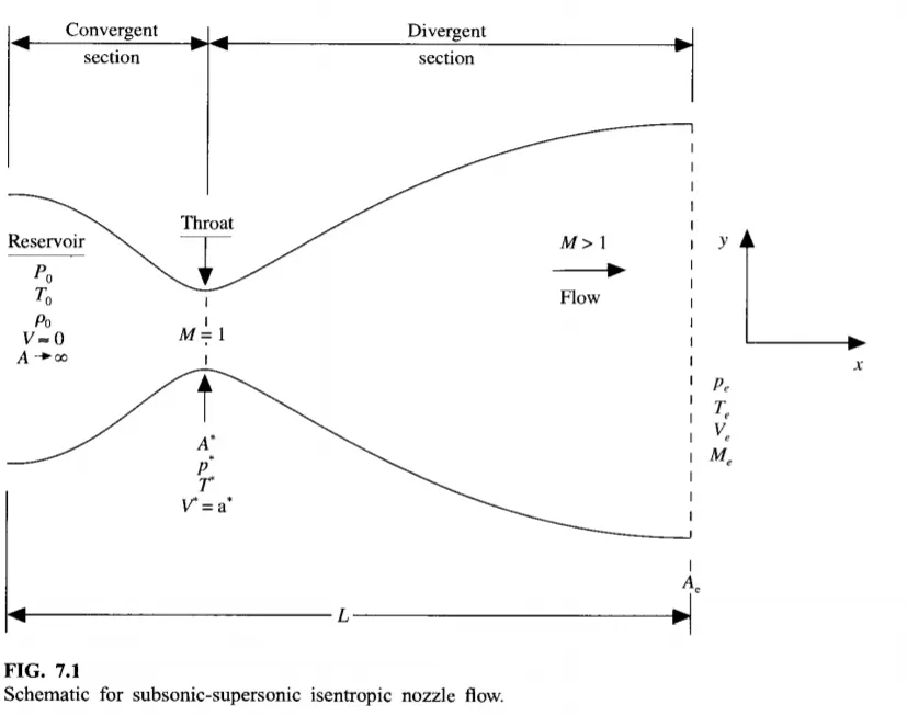
Let's examine a compact control volume within the nozzle, as depicted below.
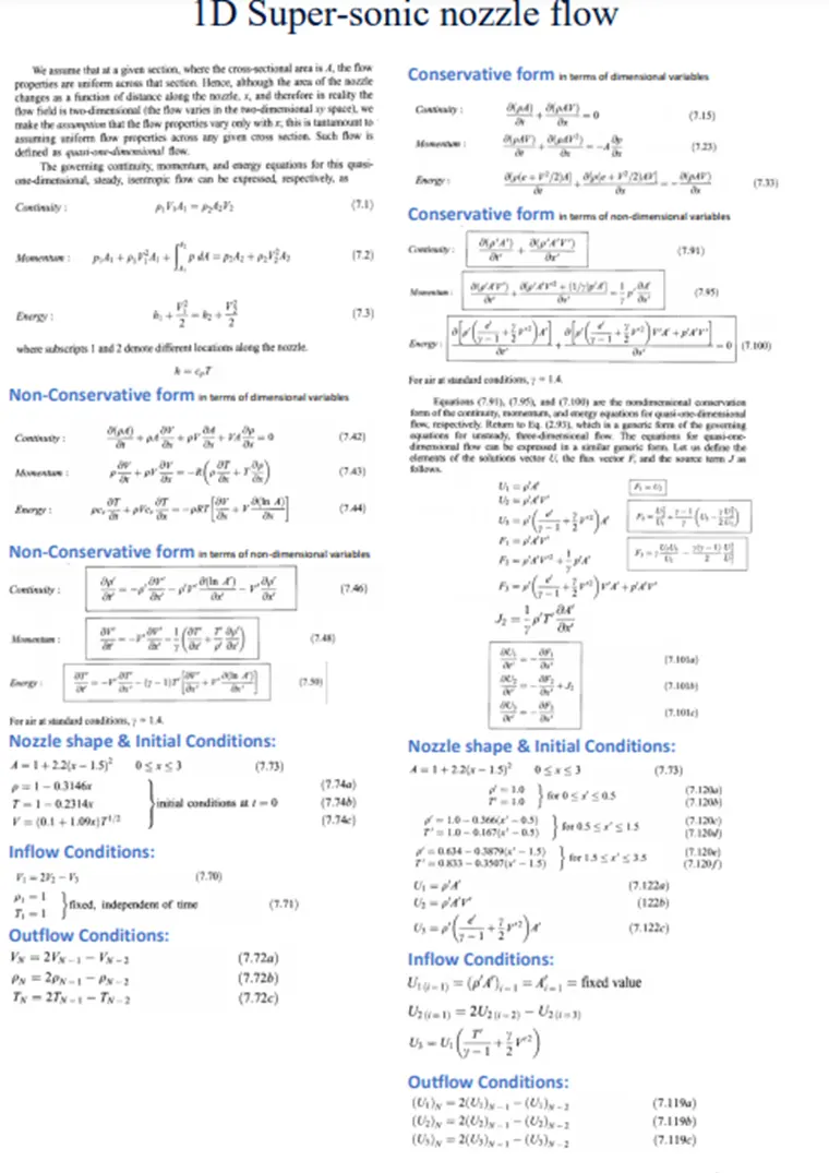
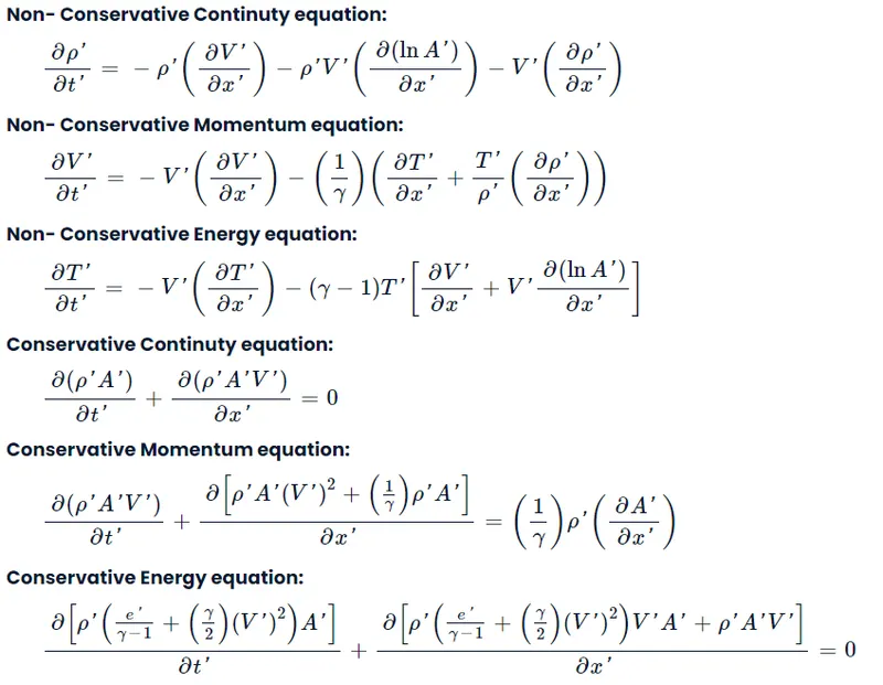
The governing continuity, momentum, and energy equations in terms of nondimensional variables for this quasi-one-dimensional, steady, and isentropic flow are as follows:
Macormack Method:
Suppose we have an equation to be solved, denoted as f(x). The subsequent steps are executed as follows:
Initial step:
Prior to commencing the calculations, it is imperative to establish the initial profiles for all flow field variables, including velocity, density, and temperature. While these are initial estimations, they should be chosen with heightened consideration for the underlying problem.
predector step:
`((del f)/(del t))_p = (f(i+1) - f(i))/(triangle x)`
Solutaion update:
`f_p = f_(Initial) + ((del f) / (del t))_p . trianglet`
`f_p =` Flow field variables calculated after the predictor step
`f_(Initial) =`flow field variable in the initial step
`triangle t` = time step size
Corrector step:
`((del f_p)/(del t) )_c =( f (i)- f(i-1))/(triangle x)`
`((del f) /(delt)) _(avg) = 0.5 (((del f)/(delt))_p + ((del f_p )/ (del t))_c)`
Final solution update:
`f_(sol) = f_(Initial) + ((del f)/(del t))_(avg) . trianglet`
`f_(sol) =`Final solution of the flow field variables for the first time step
Matlab code:
Conservative function:
clear all
close all
clc

% Inputs
n = 31;
x = linspace(0,3,n);
dx = x(2)-x(1);

% % Calculate Initial Profiles
% rho = 1-0.3146*x;
% t = 1-0.2314*x; % temperature
% v = (0.1+1.09*x).*t.^0.5;

for i = 1:n

 if x(i) <= 0.5
 rho(i) = 1;
 t(i) = 1;
 end

 if x(i)> 0.5 && x(i)<= 1.5
 rho(i) = 1 - 0.366*(x(i)-0.5);
 t(i) = 1 - 0.167*(x(i)-0.5);
 end

 if x(i)> 1.5
 rho(i) = 0.634 - 0.3879*(x(i)-1.5);
 t(i) = 0.833 - 0.3507*(x(i)-1.5);
 end

end

nt = 1400;
dt = 0.0267;
gamma = 1.4;

th = round(n/2);

% Area
a = 1+2.2*(x-1.5).^2;

v = 0.59./(rho.*a);

U1 = rho.*a;
U2 = rho.*a.*v;
U3 = U1.*(t/(gamma-1) + (gamma/2)*v.^2);

cfl = max((v+sqrt(t))*dt/dx);

% Outer Time Loop
for k = 1:nt

    U1_old = U1;
    U2_old = U2;
    U3_old = U3;

F1 = U2;
F2 = U2.^2./U1 + ((gamma-1)/gamma)*(U3 - (gamma/2)*(U2.^2./U1));
F3 = gamma*U2.*U3./U1 - 0.5*gamma*(gamma-1)*(U2.^3./U1.^2);

    % Predictor Method
    % Continuity Equation
    for j = 2:n-1


        % Continuity Equation
        dU1dt_p(j) = -(F1(j+1)-F1(j))/dx;

        J2 = (1/gamma)*rho(j)*t(j)*(a(j+1)-a(j))/dx;

        % Momentum Equation
        dU2dt_p(j) = -(F2(j+1)-F2(j))/dx + J2;

        % Energy Equation
        dU3dt_p(j) = -(F3(j+1)-F3(j))/dx;

        % Solution Update
        U1(j) = U1(j) + dU1dt_p(j)*dt;
        U2(j) = U2(j) + dU2dt_p(j)*dt;
        U3(j) = U3(j) + dU3dt_p(j)*dt;

    end
    % Predictor update
    rho = U1./a;
    t = (gamma-1)*(U3./U1 - (gamma/2)*(U2./U1).^2);

F1 = U2;
F2 = U2.^2./U1 + ((gamma-1)/gamma)*(U3 - (gamma/2)*(U2.^2./U1));
F3 = gamma*U2.*U3./U1 - 0.5*gamma*(gamma-1)*(U2.^3./U1.^2);


    % Corrector Method
    for j = 2:n-1

        % Continuity Equation
        dU1dt_c(j) = -(F1(j)-F1(j-1))/dx;

        J2 = (1/gamma)*rho(j)*t(j)*(a(j)-a(j-1))/dx;

        % Momentum Equation
        dU2dt_c(j) = -(F2(j)-F2(j-1))/dx + J2;

        % Energy Equation
        dU3dt_c(j) = -(F3(j)-F3(j-1))/dx;

    end

    % Compute the average time derivative

    dU1dt = 0.5*(dU1dt_p + dU1dt_c);
    dU2dt = 0.5*(dU2dt_p + dU2dt_c);
    dU3dt = 0.5*(dU3dt_p + dU3dt_c);

    % Final Solution Update
    for i = 2:n-1
        U1(i) = U1_old(i) + dU1dt(i)*dt;
        U2(i) = U2_old(i) + dU2dt(i)*dt;
        U3(i) = U3_old(i) + dU3dt(i)*dt;
    end

    %Final update
    rho = U1./a;
    t = (gamma-1)*(U3./U1 - (gamma/2)*(U2./U1).^2);
    v = U2./U1;

    % Apply the boundary conditions
    % Inlet Boundary Condition
    U1(1) = a(1);
    U2(1) = 2*U2(2) - U2(3);
    U3(1) = U1(1)*(t(1)/(gamma-1) + 0.5*gamma*v(1)^2);
    % Outlet Boundary Condition
    U1(n) = 2*U1(n-1) - U1(n-2);
    U2(n) = 2*U2(n-1) - U2(n-2);
    U3(n) = 2*U3(n-1) - U3(n-2);


    %Pressure
    p = rho.*t;
    %Mach no
    M = v./sqrt(t);
    %Mass flow rate
    m = rho.*a.*v;


   figure(3)
   hold on
   if k == 1
       plot(x,m);
   end
   if k == 50
       plot(x,m);
   end
   if k == 250
       plot(x,m);
   end
   if k == 500
       plot(x,m);
   end
   if k == 750
       plot(x,m);
   end
   if k == 1400
       plot(x,m);
   end

   rho_throat(k) = rho(th);
   v_throat(k) = v(th);
   t_throat(k) = t(th);
   p_throat(k) = p(th);
   M_throat(k) = M(th);

end
xlabel('Nozzle length')
ylabel('Mass flow rate')
legend('1dt','50dt','250dt','500dt','750dt','1200dt')
title('Variation of mass flow rate at different time steps')

figure(1)
subplot(5,1,1)
plot(x,v)
xlabel('Nozzle length')
ylabel('Velocity')
title('Steady state primitive variable profiles')
subplot(5,1,2)
plot(x,rho)
xlabel('Nozzle length')
ylabel('Density')
subplot(5,1,3)
plot(x,t)
xlabel('Nozzle length')
ylabel('Temperature')
subplot(5,1,4)
plot(x,p)
xlabel('Nozzle length')
ylabel('Pressure')
subplot(5,1,5)
plot(x,M)
xlabel('Nozzle length')
ylabel('Mach Number')

figure(2)
subplot(5,1,1)
plot(v_throat)
xlabel('Time step')
ylabel('Velocity')
title('Transient variation of primitive variables at throat')
subplot(5,1,2)
plot(rho_throat)
xlabel('Time step')
ylabel('Density')
subplot(5,1,3)
plot(t_throat)
xlabel('Time step')
ylabel('Temperature')
subplot(5,1,4)
plot(p_throat)
xlabel('Time step')
ylabel('Pressure')
subplot(5,1,5)
plot(M_throat)
xlabel('Time step')
ylabel('Mach Number')

figure(3)
plot(x,m);
title('Steady state mass flow rate profile')
xlabel('Nozzle length')
ylabel('Mass flow rate')
Non-Conservative function:
clear all
close all
clc

% Inputs
n = 31;
x = linspace(0,3,n);
dx = x(2)-x(1);

% Calculate Initial Profiles
rho = 1-0.3146*x;
t = 1-0.2314*x; % temperature
v = (0.1+1.09*x).*t.^0.5;

% Area
a = 1+2.2*(x-1.5).^2;
nt = 1400;
dt = 0.04;
gamma = 1.4;

th = round(n/2);

cfl = max((v+sqrt(t))*dt/dx);

% Outer Time Loop
for k = 1:nt

    rho_old = rho;
    v_old = v;
    t_old = t;

    % Predictor Method
    % Continuity Equation
    for j = 2:n-1
        dvdx = (v(j+1)-v(j))/dx;
        drhodx = (rho(j+1)-rho(j))/dx;
        dtdx = (t(j+1)-t(j))/dx;
        dlogadx = (log(a(j+1))-log(a(j)))/dx;

        % Continuity Equation
        drhodt_p(j) = -rho(j)*dvdx - rho(j)*v(j)*dlogadx-v(j)*drhodx;

        % Momentum Equation
        dvdt_p(j) = -v(j)*dvdx-(1/gamma)*(dtdx+(t(j)/rho(j))*drhodx);

        % Energy Equation
        dtdt_p(j) = -v(j)*dtdx-(gamma-1)*t(j)*(dvdx+v(j)*dlogadx);

        % Solution Update
        rho(j) = rho(j) + drhodt_p(j)*dt;
        v(j) = v(j) + dvdt_p(j)*dt;
        t(j) = t(j) + dtdt_p(j)*dt;
    end

    % Corrector Method
for j = 2:n-1
        dvdx = (v(j)-v(j-1))/dx;
        drhodx = (rho(j)-rho(j-1))/dx;
        dtdx = (t(j)-t(j-1))/dx;
        dlogadx = (log(a(j))-log(a(j-1)))/dx;

        % Continuity Equation
        drhodt_c(j) = -rho(j)*dvdx - rho(j)*v(j)*dlogadx-v(j)*drhodx;

        % Momentum Equation
        dvdt_c(j) = -v(j)*dvdx-(1/gamma)*(dtdx+(t(j)/rho(j))*drhodx);

        % Energy Equation
        dtdt_c(j) = -v(j)*dtdx-(gamma-1)*t(j)*(dvdx+v(j)*dlogadx);

    end

    % Compute the average time derivative

    drhodt = 0.5*(drhodt_p + drhodt_c);
    dvdt = 0.5*(dvdt_p + dvdt_c);
    dtdt = 0.5*(dtdt_p + dtdt_c);

    % Final Solution Update
    for i = 2:n-1
        rho(i) = rho_old(i) + drhodt(i)*dt;
        v(i) = v_old(i) + dvdt(i)*dt;
        t(i) = t_old(i) + dtdt(i)*dt;
    end

    % Apply the boundary conditions
    % Inlet Boundary Condition
    v(1) = 2*v(2) - v(3);
    % Outlet Boundary Condition
    v(n) = 2*v(n-1) - v(n-2);
    rho(n) = 2*rho(n-1) - rho(n-2);
    t(n) = 2*t(n-1) - t(n-2);

    %Pressure
    p = rho.*t;
    %Mach no
    M = v./sqrt(t);
    %Mass flow rate
    m = rho.*a.*v;

   figure(3)
   hold on
   if k == 1
       plot(x,m);
   end
   if k == 50
       plot(x,m);
   end
   if k == 250
       plot(x,m);
   end
   if k == 500
       plot(x,m);
   end
   if k == 750
       plot(x,m);
   end
   if k == 1400
       plot(x,m);
   end

   rho_throat(k) = rho(th);
   v_throat(k) = v(th);
   t_throat(k) = t(th);
   p_throat(k) = p(th);
   M_throat(k) = M(th);

end
xlabel('Nozzle length')
ylabel('Mass flow rate')
legend('1dt','50dt','250dt','500dt','750dt','1200dt')
title('Variation of mass flow rate at different time steps')

%plotting
figure(1)
subplot(5,1,1)
plot(x,v)
xlabel('Nozzle length')
ylabel('Velocity')
title('Steady state primitive variable profiles')
subplot(5,1,2)
plot(x,rho)
xlabel('Nozzle length')
ylabel('Density')
subplot(5,1,3)
plot(x,t)
xlabel('Nozzle length')
ylabel('Temperature')
subplot(5,1,4)
plot(x,p)
xlabel('Nozzle length')
ylabel('Pressure')
subplot(5,1,5)
plot(x,M)
xlabel('Nozzle length')
ylabel('Mach Number')

figure(2)
subplot(5,1,1)
plot(v_throat)
xlabel('Time step')
ylabel('Velocity')
title('Transient variation of primitive variables at throat')
subplot(5,1,2)
plot(rho_throat)
xlabel('Time step')
ylabel('Density')
subplot(5,1,3)
plot(t_throat)
xlabel('Time step')
ylabel('Temperature')
subplot(5,1,4)
plot(p_throat)
xlabel('Time step')
ylabel('Pressure')
subplot(5,1,5)
plot(M_throat)
xlabel('Time step')
ylabel('Mach Number')

figure(3)
plot(x,m);
title('Steady state mass flow rate profile')
xlabel('Nozzle length')
ylabel('Mass flow rate')
Output:
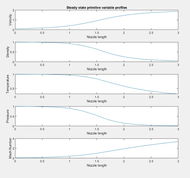
STEADY-STATE VALUES OF FLOW FIELD VARIABLES:
Conservative form:
Non - Conservative form:
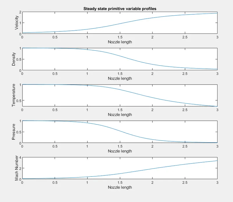
When compared to the analytical answer from Anderson Textbook, the figures above are almost identical. The figures above show that while velocity and Mach Number rise from intake to outlet, pressure, density, and temperature decrease along the same route from inlet to outlet. Because of energy conservation, an increase in velocity in horizontal flow must be followed by a drop in pressure, according to Bernoulli's equation. The energy required to raise the velocity of the fluid is at the price of static pressure energy.
The most crucial parameter for understanding in this case is the Mach Number. Mach Number rises as the value of x rises.
Mach number = speed of object / speed of sound
VARIATION OF MASS FLOW RATE DISTRIBUTION INSIDE THE NOZZLE :
Non-Conservative form:
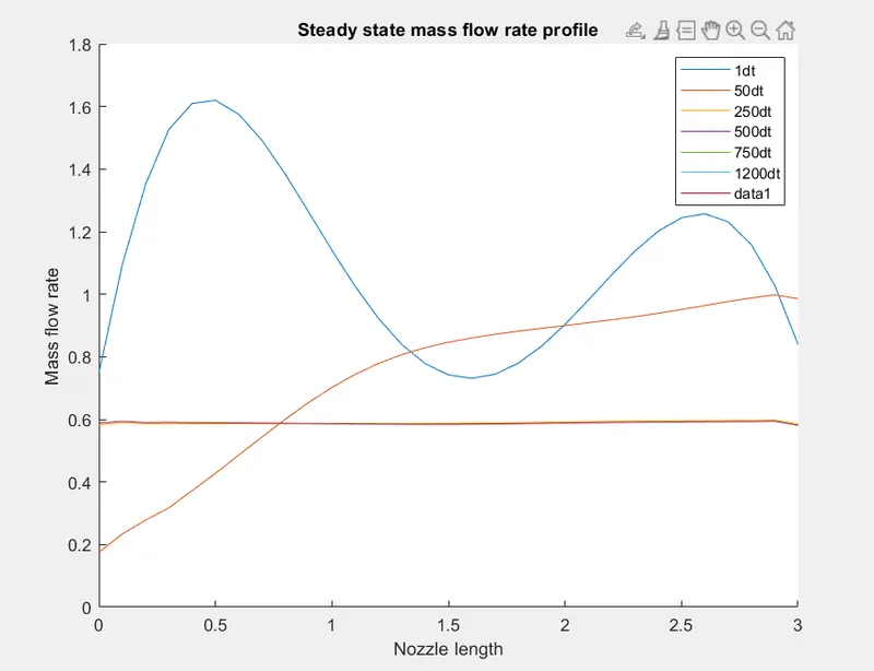
During the time-marching method, the non-dimensional mass flow is plotted as a function of non-dimensional distance through the nozzle at different time steps in the graph. The first two curves show the evolution of the profile under beginning conditions. We can observe that the flow obtains an essentially constant mass flow profile after 250 iterations.
Conservative form:
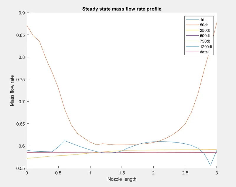
1. The conservative and non-conservative forms have distinct beginning circumstances, resulting in a different mass flow rate curve in the non-conservative form analysis.
2. The curves are closer to each other and to their analytical value of 0.579, indicating that the conservative form retains more mass than the non-conservative version.
TIME-WISE VARIATION OF VARIOUS PRIMITIVE VARIABLES AT THE THROAT:
Non-Conservative form:
Conservative form:
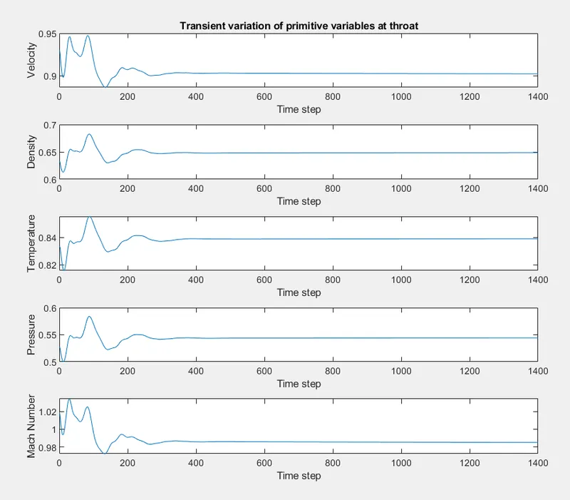
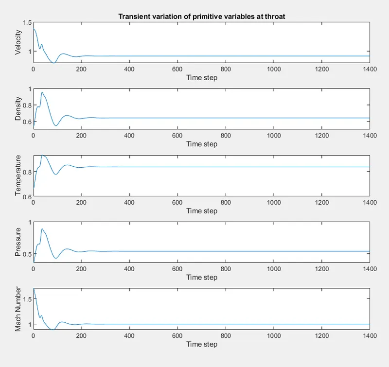
The figures above show that the time-wise modulation of non-dimensional flow field variables at the neck reaches the steady-state in both non-conservative and conservative forms. We can also see that the oscillations gradually settle down to a stable state. Here, we can see that the non-conservative form reaches a steady state after around 200 timesteps, but the conservative form takes roughly 300 timesteps to reach a steady state since the oscillations last a little longer in its case. As a result, the non-conservative version achieves steady-state faster than the conservative form.
Grid independence test:
|
Parameters |
Exact analytical solution |
Non-Conservative Form |
Conservative Form |
||
|
n = 31 |
n = 61 |
n = 31 |
n = 61 |
||
|
rho (ρ) |
0.636 |
0.6396 |
0.6376 |
0.6437 |
0.6375 |
|
T |
0.835 |
0.8368 |
0.8354 |
0.8365 |
0.8347 |
|
p |
0.531 |
0.5353 |
0.5327 |
0.5385 |
0.5321 |
|
Mach number (M) |
1 |
0.9988 |
0.9996 |
0.9942 |
1.006 |
|
Mass Flow Rate (m) |
0.583 |
0.5844 |
0.5826 |
0.5854 |
0.5828 |
To perform a grid dependence test, two scenarios are considered: one with 31 grid points and the other with 61 grid points.
- From the table, we can see that as the number of grid points rises, so does the solution accuracy, and the non-conservative version outperforms the conservative form. The following table also shows that the values for both forms are almost same, as are all of the primitive variables, even when the grid points are altered from 31 to 61.
CONCLUSIONS:
- The conservation form produces a more uniform mass flow distribution. It is superior at maintaining mass across the flow field because mass flow is one of the dependent variables in the equations, and mass flow rate is the major outcome generated from the conservation-form equations. In the non-conservation version of the equations, the dependent variables are primitive variables, and the mass flow is found only as a secondary consequence.
- In terms of accuracy, neither form clearly outperforms the other, though the non-conservation form appears to produce slightly more accurate results for the flow field variables/primitive variables and the conservation form appears to produce slightly more accurate results for the flux variables.
- Non-conservation form results in fewer residuals, and the amount by which the residuals decay is frequently used as an indicator of the numerical algorithm's quality. As a result, we know that the non-conservation variant performs better.
Reference:
The governing equations, Boundary and initial conditons are taken from the CFD by John D Anderson