Week 5 - Genetic Algorithm

Aim:

To find the global maxima of the stalagmite function using Genetic Algorithm in MATLAB.

Objective:

The objective of the challenge is to write a report that consist of step wise explanation of your code, errors faced while programming, the steps to overcome those errors and good presentaion of the code with line by line explanation.

1. To write a code in MATLAB to optimise the stalagmite function and find the global maxima of the function.
2. Clearly expalin the concept of genetic algorithm in your own words and also explain the syntax for ga in MATLAB in your report.
3. Make sure that your code gives the same output, even if it is made to run several times.
4. Plot graphs for all 3 studies and for F maximum vs no. of iterations. Title and axes labels are a must, legends could be shown if necessary.

Theory:

Genetic Algorithm:

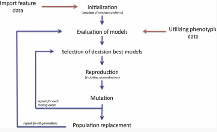
Genetic algorithm (GA) is search-based optimization technique based on the principles of Genetics and natural selection. It is used to find optimum solution of complicated problem, which otherwise take very long time to solve. Whatever solutions are available, they are combined or modified to get better and better solutions. It uses techniques such as selection, mutation, inheritance, and recombination to solve problem. In genetic algorithm group of individuals is created randomly from given population. In GA population represents all possible solutions that given problem can have.

• The genetic algorithm is an algorithm used for solving both constrained and unconstrained optimization problems.
• A genetic algorithm is a search heuristic that is inspired by Charles Darwin’s theory of natural evolution.
• It selects random inputs called as population, check their fitness for selection and pairing purposes (the pair is called as parents) to generate new data (called as new/next generation).
• This next generation data is mutated from data acquired from parents which is essential for computing optimised output.

Advantages of GA

• Faster and more efficient method compared to other methods available
• It gives all possible solutions or outputs for given inputs
• It can be used to find out solution of complicated problem which otherwise takes very long time to solve.
• Useful when possible no. of solutions is very large.

Basic steps in genetic algorithm

• Start with initial population
• Selection of parent candidate’s solutions for mating.
• Crossover and mutations are applied to generate new candidate solutions.
• Determination of fitness of new candidate solution.
• Replacement of existing solution candidates with better solutions got in previous step.
• Repetition of above process till optimum solution is got.

Genetic algorithm syntax in MATLAB

ga(@stalagmite_fun,2)

Above is the syntax to determine minimum value of a function using MATLAB. Here ‘GA’ represents genetic algorithm, stalagmite_fun is the function name and 2 represents no. of varaibales.

In general it is of the form “x = ga(fun,nvars)”.

x = ga(fun,nvars,A, b,Aeq,beq,lb,ub)

above syntax defines or specifies upper and lower bounds of a variable x so that solution will be such that x lies between upper (ub) and lower bound (lb)

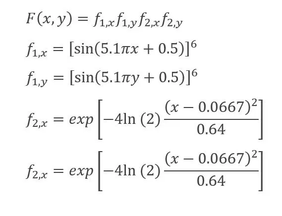
Governing equation:

Program code:

% The stalagmite function
function [stalagmite] = stalagmite_fun(input_vector)
    x = input_vector(1);
    y = input_vector(2);
    f1x = (sin((5.1*pi*x)+0.5))^6; % term 1
    f1y = (sin((5.1*pi*y)+0.5))^6; % term 2
    f2x = exp((-4*log(2)*(x-0.0667)^2)/0.64); % term 3
    f2y = exp((-4*log(2)*(y-0.0667)^2)/0.64); % term 4
    
    stalagmite = -(f1x*f1y*f2x*f2y);
end

1. Case 1 - Unbounded inputs and default population

% Program to find global maxima using genetic algorithm
close all
clear all
clc
% Field of interest of optimisation
x = linspace(0,0.6,150);
y = linspace(0,0.6,150);
num_cases =50;
[xx yy] = meshgrid(x,y);
% Creating Data points of stalagmite Function
for i = 1:length(xx)
    for j = 1:length(yy)
        input_vector(1) = xx(i,j);
        input_vector(2) = yy(i,j);
        f(i,j) = stalagmite_fun(input_vector);
    end
end
% Iterations of genetic algorithm
tic
for i = 1:num_cases
    [inputs, fopt(i)] = ga(@stalagmite_fun,2);
    xopt(i) = inputs(1);
    yopt(i) = inputs(2);
end
toc
% Ploting results
figure(1)
subtitle('Genetic Algorithm Unbound Inputs')
subplot(2,1,1)
hold on
surfc(xx,yy,-f)
shading interp
title('Genetic Algorithm Unbound Inputs')
plot3(xopt,yopt,-fopt,'marker','o','markersize',5)
xlabel('x axis')
ylabel('y axis')
zlabel('f(x,y)')
subplot(2,1,2)
plot(-fopt)
xlabel('Iterations')
ylabel('Global Maxima')
title('Global Maxima vs Iterations')
axis([0 50 0 1.5])

2. Case 2 - Bound inputs and default population

% Program to find global maxima using genetic algorithm
close all
clear all
clc
% Field of interest of optimisation
x = linspace(0,0.6,150);
y = linspace(0,0.6,150);
num_cases =50;
[xx yy] = meshgrid(x,y);
% Creating Data points of stalagmite Function
for i = 1:length(xx)
    for j = 1:length(yy)
        input_vector(1) = xx(i,j);
        input_vector(2) = yy(i,j);
        f(i,j) = stalagmite_fun(input_vector);
    end
end


% Defining Population size
options = optimoptions('ga');
options = optimoptions(options, 'PopulationSize',250);

% Iterations of genetic algorithm Bound Inputs
tic
for i = 1:num_cases
    [inputs, fopt(i)] = ga(@stalagmite_fun,2,[],[],[],[],[0;0],[0.6;0.6]); % Bound Inputs
    xopt(i) = inputs(1);
    yopt(i) = inputs(2);
end
toc
% Ploting results
figure(1)
subtitle('Genetic Algorithm Bound Inputs')
subplot(2,1,1)
hold on
surfc(xx,yy,-f)
shading interp
title('Genetic Algorithm Bound Inputs')
plot3(xopt,yopt,-fopt,'marker','o','markersize',5)
xlabel('x axis')
ylabel('y axis')
zlabel('f(x,y)')
subplot(2,1,2)
plot(-fopt)
xlabel('Iterations')
ylabel('Global Maxima')
title('Global Maxima vs Iterations')
axis([0 50 0 1.5])

3. Case 3 - Bound Inputs and 400 population

% Program to find global maxima using genetic algorithm
close all
clear all
clc
% Field of interest of optimisation
x = linspace(0,0.6,150);
y = linspace(0,0.6,150);
num_cases =50;
[xx yy] = meshgrid(x,y);
% Creating Data points of stalagmite Function
for i = 1:length(xx)
    for j = 1:length(yy)
        input_vector(1) = xx(i,j);
        input_vector(2) = yy(i,j);
        f(i,j) = stalagmite_fun(input_vector);
    end
end


% Defining Population size
options = optimoptions('ga');
options = optimoptions(options, 'PopulationSize',250);

% Iterations of genetic algorithm Bound Inputs
tic
for i = 1:num_cases
    [inputs, fopt(i)] = ga(@stalagmite_fun,2,[],[],[],[],[0;0],[0.6;0.6]); % Bound Inputs
    xopt(i) = inputs(1);
    yopt(i) = inputs(2);
end
toc
% Ploting results
figure(1)
subtitle('Genetic Algorithm Bound Inputs')
subplot(2,1,1)
hold on
surfc(xx,yy,-f)
shading interp
title('Genetic Algorithm Bound Inputs')
plot3(xopt,yopt,-fopt,'marker','o','markersize',5)
xlabel('x axis')
ylabel('y axis')
zlabel('f(x,y)')
subplot(2,1,2)
plot(-fopt)
xlabel('Iterations')
ylabel('Global Maxima')
title('Global Maxima vs Iterations')
axis([0 50 0 1.5])

Explanation:

1. First, Linspace command is used to define x & y with 150 elements between zero and 0.6 including the bounds.
2. Then num_cases is set which will be used as counter for iteration to 50
3. then a 2D grid is made using meshgrid command is created from x & y input tobe output to xx & yy
4. then for loop is used to solve the genetic algorithm for every element in the 2D mesh grid
5. the length of rows & column (which have equal length) are used as counters
6. then the input vector is declared as ga requires input vector which is each value in the mesh grid
7. then output of stalagmite function is stored in matrix
8. then tic command is used to start a timer
9. then for loop bounded by the number of iterations is formed
10. then ga code is entered for unbounded statistical study which have the following format :

11. Then smallest (minimum) value of the function for each iteration is output & its x & y coordinates which are stored in seperate variables
12. then 'toc' command is used to stop the timer and the output is stored in study_time1
13. then figure1 is plotted by the following steps-
14. First subplot command is used to partition the plot window in order to draw more than one plot in the same window, two rows and one column are specified and then the position of each plot is selected
15. then hold on command is used to prevent plot for being removed
16. the surfc command is used to plot contour with xx & yy value from the mesh grid as input and negative optimum value is used because we need to maximize the function
17. then x,y,& z axis are labelled
18. then shading interp is used to smoothen the function plot and to remove the grid lines
19. then plot 3 command is used to plot a point in 3D, here it will plot- fopt because we need the maximum value of the function not the minimum
20. then the graph title is selected
21. then fopt value of the function is plotted on the second plot in the second row
22. then its x & y axis are labelled.
23. then the same study is made but this time it is bounded (has lower & upper limit) which requires the same commands and step excepts the ga command which have the following format
24. the range of the genetic algorithm is bounded by introducing values for lower and upper bounds and hence the values of global maxima and the values of x & y will be within the defined search space in inputs
25. then increasing population size study was done which is the same as before but it had different ga code of :

26. the range of the genetic algorithm is bounded as in study-2 but to improove the accuracy, the commands optimoptions is introduced to increase the Population Size
27. then total time is computed
28. then using fprintf command the results are printed in the command windows
29. then the study time is printed
30. then x, y coordinate of the maximum optimum values are printed
31. then the optimum values of the function (maximum value) is printed which is calculated from the (negative mean) of the all iterations of the output value and the negative sign is used to get the maximum value
32. then the study time of the whole 3 studies combined is printed.

Output:

Case 1:

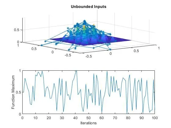
Case 2:

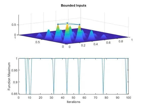
Case 3:

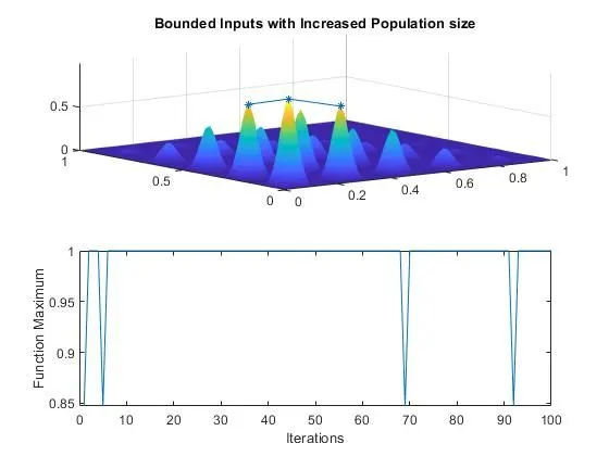
Error occured:

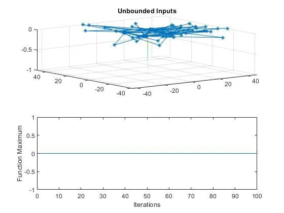
1. The plots obtained were not proper because ‘ga’ function is used to find minima but we have to find maxima so we have to introduce negative sign in function code in function definition line.