Challenge

Week 7 - Simulation of a 1D Supersonic nozzle flow simulation using Macormack Method

SSridhar Kumar5 Jun 2023

1D SUPERSONIC NOZZLE FLOW SIMULATION USING MacCORMACK's METHOD

AIM:

To simulate the isentropic flow through a quasi 1D subsonic-supersonic nozzle and derive both the conservative and non-conservative forms of the governing equations and sovle them using the MacCormack's technique.

OBJECTIVE
1. Steady-state distribution of primitive variables inside the nozzle
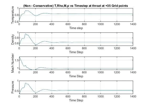
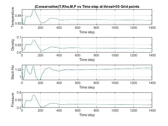
2. Time-wise variation of the primitive variables
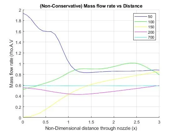
3. Variation of Mass flow rate distribution inside the nozzle at different time steps during the time-marching process
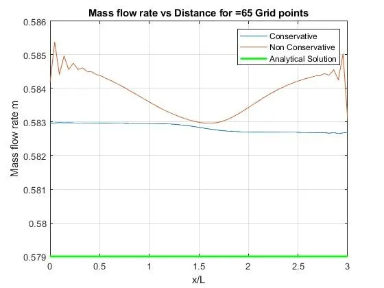
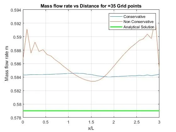
4. Comparison of Normalized mass flow rate distributions of both forms

THEORY

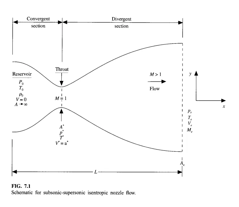
Consider an isentropic flow through a convergent-divergent nozzle with length L or x

	Variables at Inlet	Variables at throat	Variables at Exit
Pressure	`P_o`	P`	`P_e`
Temperature	`T_o`	T`	`T_e`
Velocity	`V_o`	V`	`V_e`
Area	`A_o`	A`	`A_e`
Mach Number	M<1	M=1	M>1

Governing Equations for Quasi-One -Dimesional Flow:

The mach number variation along the nozzle is exclusively governed by the below equation

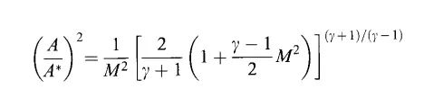
where `gamma=C_p/C_v=1.4` for standard conditions of air.

Similarly , equations for variation in pressure , density and temperature are given below;

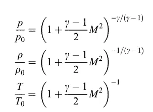
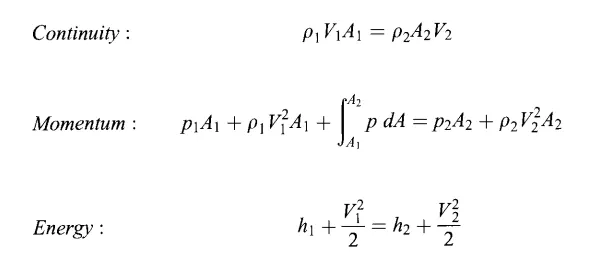
Since the quasi-one-dimensional assumption twists certain aspects of physics , we take the integral form of governing equations and work with them so that the physical aspects remain true . Hence we can re-write the governing equations in following manner

Governing equations :

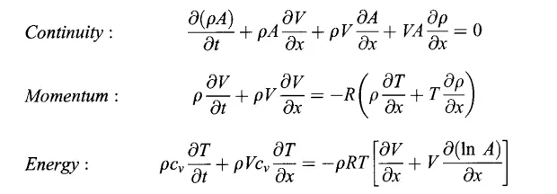
Governing equations in conservative form

Continuity Equation

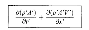
Momentum Equation

Energy Equation

Governing equations in non-conservative form,

Maccarmack method:

* In CFD, the MacCormack method is a widely used discretization scheme for the numerical solution of hyperbolic partical differential equations.

* This second-order finite different method was introduced by Robert W. MacCormack in 1969.

* The MacCormack method is elegant and easy to understand and program.

* The MacCormack method is a variation of the two step lax wendroff scheme but is much simpler in application.

Predictor step:

* In the predictor step, a "provisional" value of at time level (denoted by ) is estimated as follows.The above equation is obtained by replacing the spatial and temporal derivatives in the previous

first order hyperbolic equation using forward difference.

Corrector step:

* In the corrector step, the predicted value is corrected according to the equation.

* Note that the corrector step uses backward finite different method approximations for spatial derivative. The time-step used in the corrector step is in contrast to the used in the predictor step.

Replacing the term by the temporal average.

While looking at the diagram ,we can observe that the inlet and outlet variables depend on time rate of change of velocities,

Hence we use Von-Neumann boundary conditions .

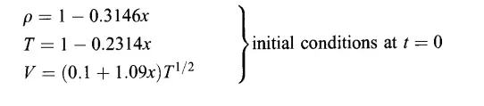
In non-conservative form, we consider the following initial and boundary conditions

initial condition

Boundary condition at inlet,

At Outlet,

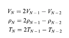
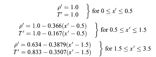
In conservative form , we use following initial conditions ,

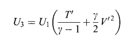
Boundary Condition at Inlet,

At Outlet,

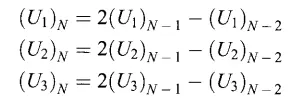
where N=i.

Discretization scheme used

By MacCormack's Method ,

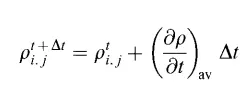
where ,`rho_(i,j)^(t+trianglet)` is the density at next time step

`rho_(i,j)^t` is the density at present time step

`((delrho)/(delt))_(av)` is the partial derivative of density obtained from predictor and corrector step

`trianglet` is the time step.

Equations for predictor and corrector step are given below,

predictor step:

Equation for density by replacing partial differences with forward differences,

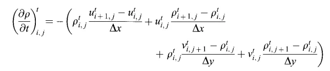
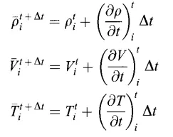
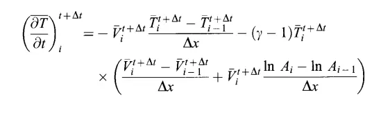
Using above method , we obtain equation for predicted density, velocity and temperature at next time step

Corrector step,

Equation for density by replacing partial derivatives with rearward differences ,

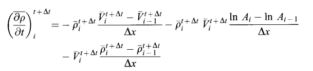
Similarly we can apply for temperature and velocity as well

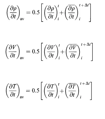
Equation for average calculation,

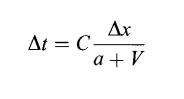
Equation for time step,

Hence we can obtain solution for density , velocity and temperature by applying all the above values in first equation under MacCormacks method.

Function for Conservative Form,

% Writing Function for conservative form

function[rho_c,v_c,t_c,M_c,p_c,m_c,p_tc,rho_tc,t_tc,M_tc] = conservative(n,nt)

x=linspace(0,3,n);
% gamma denoted as w
w = 1.4;
dx = x(2)-x(1);

% Area
a=1+(2.2*(x-1.5).^2);

for i=1:length(x)

    if(x(i)>=0)&&(x(i)<=0.5)
        rho(i) = 1;
        t(i) = 1;

    elseif(x(i)>=0.5)&&(x(i)<=1.5)

        rho(i) = 1-0.366.*(x(i)-0.5);
        t(i) = 1-0.167.*(x(i)-0.5);
    else
        rho(i) =0.634-0.3879.*(x(i)-1.5);
        t(i)=0.833-0.3507.*(x(i)-1.5);
    end
end
a=1+(2.2*(x-1.5).^2);
v=(0.59)./(rho.*a);

% Defining the initial solution variables
U1=rho.*a;
U2=rho.*a.*v;
U3=rho.*((t./(w-1)) + ((w/2).*v.^2)).*a;

% Defining the timestep
delta_t = 0.5*(dx./(sqrt(t)+v));
dt=min(delta_t);

% Defining the time loop
for k=1:nt

%Defining the old values
    U1_old=U1;
    U2_old=U2;
    U3_old=U3;
% Calculating the flux values
    F1=U2;
    F2=((U2.^2)./U1)+((w-1)/w)*(U3-(w/2)*((U2.^2)./U1));
    F3=(w*(U2.*U3)./U1)-((w*(w-1))/2)*((U2.^3)./(U1.^2));


%Predictor
for j=2:n-1

%source term
    J(j)=(1/w)*rho(j)*t(j)*((a(j+1)-a(j))/dx);

% Continuity Equation
    dU1dt_p(j)=-((F1(j+1)-F1(j))/dx);

% Momentum Equation
    dU2dt_p(j)=-((F2(j+1)-F2(j))/dx)+J(j);

% Energy Equation
    dU3dt_p(j)=-((F3(j+1)-F3(j))/dx);

% Update the solution vector
    U1(j)=U1_old(j)+(dU1dt_p(j))*dt;
    U2(j)=U2_old(j)+(dU2dt_p(j))*dt;
    U3(j)=U3_old(j)+(dU3dt_p(j))*dt;
end

rho=U1./a;
v=U2./U1;
t=(w-1)*((U3./U1)-((w/2)*(v.^2)));

% Updating the flux terms
F1=U2;
F2=((U2.^2)./U1)+((w-1)/w)*(U3-(w/2)*((U2.^2)./U1));
F3=(w*(U2.*U3)./U1)-((w*(w-1))/2)*((U2.^3)./(U1.^2));


%Corrector step
for q=2:n-1

%Defining the soource terms
    J(q)=(1/w)*rho(q)*t(q)*((a(q)-a(q-1))/dx);

% Continuity Equation
    dU1dt_c(q)=-((F1(q)-F1(q-1))/dx);

%Momentum Equation
    dU2dt_c(q)=-((F2(q)-F2(q-1))/dx)+J(q);
    
% Energy Eqution
    dU3dt_c(q)=-((F3(q)-F3(q-1))/dx);

end

% Compute the Average values
    dU1dt_av=0.5*(dU1dt_p+dU1dt_c);
    dU2dt_av=0.5*(dU2dt_p+dU2dt_c);
    dU3dt_av=0.5*(dU3dt_p+dU3dt_c);

%  Calculating the final solution
    for m=2:n-1

        U1(m)=U1_old(m)+(dU1dt_av(m)*dt);
        U2(m)=U2_old(m)+(dU2dt_av(m)*dt);
        U3(m)=U3_old(m)+(dU3dt_av(m)*dt);
    end

%defining boundary condition at Inlet
U1(1)=rho(1)*a(1);
U2(1)=2*U2(2)-U2(3);
v(1)=U2(1)/U1(1);
U3(1)=U1(1)*(t(1)/(w-1)+(w/2)*v(1)^2);

%defining boundary condition at Outlet
U1(n)=2*U1(n-1)-U1(n-2);
U2(n)=2*U2(n-1)-U2(n-2);
U3(n)=2*U3(n-1)-U3(n-2);

rho=U1./a;
v=(U2./U1);
t=(w-1)*((U3./U1)-(w/2)*(U2./U1).^2);

%Mach Number
M=(v./sqrt(t));

% Pressure
p=rho.*t;

% Mass flow rate
m=rho.*v.*a;

% Calculating variables at the throttle
throat=find(a==1);
p_t(k)=p(throat);
rho_t(k)=rho(throat);
t_t(k)=t(throat);
M_t(k)=M(throat);

% Plotting the non dimensional mass flow at different time step
figure(6)

hold on
if k==50
    plot(x,m,'b')
elseif k==100
    plot(x,m,'g')
elseif k==150
    plot(x,m,'y')
elseif k==200
    plot(x,m,'m')
elseif k==700
    plot(x,m,'c')

% Labelling
    title('(Conservative) Mass flow rate vs Distance')
    legend('50','100','150','200','700')
    xlabel('Non-Dimensional distance through nozzle (x)')
    ylabel('Mass flow rate (rho.A.V)')
    grid on
end

end

rho_c=rho;
v_c=v;
t_c=t;
M_c=M;
p_c=p;
m_c=m;
p_tc=p_t;
rho_tc=rho_t;
t_tc=t_t;
M_tc=M_t;

end

Function for Non-Conservative Form

% Writing Function for Non conservative form

function[rho,v,t,M,p,m,p_t,rho_t,t_t,M_t] = non_conservative(n,nt)

x=linspace(0,3,n);
% gamma denoted as w
w = 1.4;
dx = x(2)-x(1);

rho=1-0.3146*x;
% Temperature
t=1-0.2314*x;
v=(0.1+1.09*x).*t.^0.5;

% Area
a=1+(2.2*(x-1.5).^2);

% Timesteps
nt=1400;
dt=0.02;

delta_t=0.5*(dx./(sqrt(t)+v));

dt=min(delta_t);


% Outer time Loop
for k=1:nt

%Predictor step

rho_old=rho;
v_old=v;
t_old=t;

% Defining the timeloop

for j=2:n-1

    dvdx=(v(j+1)-v(j))/dx;
    drhodx=(rho(j+1)-rho(j))/dx;
    dtdx=(t(j+1)-t(j))/dx;
    dlogadx=(log(a(j+1))-log(a(j)))/dx;

%Continuity Equation
drhodt_p(j)=-rho(j)*dvdx - rho(j)*v(j)*dlogadx-v(j)*drhodx;

% Momentum Equation
dvdt_p(j) = -v(j)*dvdx - ((1/w)*(dtdx+(t(j)/rho(j)*drhodx)));

% Energy Equatiion
dTdt_p(j) = -v(j)*dtdx-(w-1)*t(j)*(dvdx+v(j)*dlogadx);

% Update the solution

v(j) = v(j)+dvdt_p(j)*dt;
rho(j)=rho(j)+drhodt_p(j)*dt;
t(j)=t(j)+dTdt_p(j)*dt;
end

% Corrector Method
for j=2:n-1

dvdx=(v(j)-v(j-1))/dx;
drhodx=(rho(j)-rho(j-1))/dx;
dtdx=(t(j)-t(j-1))/dx;
dlogadx=(log(a(j))-log(a(j-1)))/dx;

%Continuity Equation
drhodt_c(j)=-rho(j)*dvdx - rho(j)*v(j)*dlogadx-v(j)*drhodx;

% Momentum Equation
dvdt_c(j) = -v(j)*dvdx - ((1/w)*(dtdx+(t(j)/rho(j)*drhodx)));

% Energy Equatiion
dTdt_c(j) = -v(j)*dtdx-(w-1)*t(j)*(dvdx+v(j)*dlogadx);

end

% Compute Average
drhodt_a=0.5*(drhodt_p+drhodt_c);
dvdt_a=0.5*(dvdt_p+dvdt_c);
dTdt_a=0.5*(dTdt_p+dTdt_c);

for i=2:n-1
    v(i)=v_old(i)+dvdt_a(i)*dt;
    rho(i)=rho_old(i)+drhodt_a(i)*dt;
    t(i)=t_old(i)+dTdt_a(i)*dt;
end

% Boundary Condition at the inlet
v(1) =2*v(2)-v(3);

% Outlet
v(n)=2*v(n-1) - v(n-2);
t(n)=2*t(n-1)-t(n-2);
rho(n)=2*rho(n-1)-rho(n-2);

% Mach Number
M=(v./sqrt(t));

% Density
p=rho.*t;

% Mass flow
m=rho.*v.*a;

throat = find(a==1);
p_t(k)=p(throat);
rho_t(k)=rho(throat);
t_t(k)=t(throat);
M_t(k)=M(throat);


figure(5)

hold on
if k==50
    plot(x,m,'b')
elseif k==100
    plot(x,m,'g')
elseif k==150
    plot(x,m,'y')
elseif k==200
    plot(x,m,'m')
elseif k==700
    plot(x,m,'c')
    title('(Non-Conservative) Mass flow rate vs Distance')
    legend('50','100','150','200','700')
    xlabel('Non-Dimensional distance through nozzle (x)')
    ylabel('Mass flow rate (rho.A.V')
end

end

end

MATLAB for 1D Supersonic Nozzle flow simulation using MacCormack's Method,

%MATLAB Code For 1D Supersonic Nozzle Flow Simulation using Macormack Method

clear all
close all
clc

n=input('Enter number of grid points');
x=linspace(0,3,n);
w=1.4;
dx=x(2)-x(1);

% Area
a=1+(2.2*(x-1.5).^2);

% Timestep
nt=1400;

%Non-Conservative Form
[rho,v,t,M,p,m,p_t,rho_t,t_t,M_t]=non_conservative(n,nt);

% Conservative Form
[rho_c,v_c,t_c,M_c,p_c,m_c,p_tc,rho_tc,t_tc,M_tc] = conservative(n,nt);

% Non_Conservative
% Plot Variable vs Distance
figure(1)
subplot(4,1,1)
plot(x,M)
title_text=sprintf('(Non-Conservative) Dimensionless M,P,Rho,T vs Distance (No.of Timestep=%d)',nt);
title(title_text)
xlabel('Distance')
ylabel('Mach Number')
hold on

subplot(4,1,2)
plot(x,p)
xlabel('Distance')
ylabel('Pressure')
hold on

subplot(4,1,3)
plot(x,rho)
xlabel('Distance')
ylabel('Density')
hold on

subplot(4,1,4)
plot(x,t)
xlabel('Distance')
ylabel('Temperature')
hold on


figure(2)
nt=1:1400;
subplot(4,1,1)
plot(nt,t_t)
title_text=sprintf('(Non - Conservative) T,Rho,M,p vs Timestep at throat at =%d Grid points ',n)
title(title_text)
xlabel('Time step')
ylabel('Temperature')
hold on

subplot(4,1,2)
plot(nt,rho_t)
xlabel('Time Step')
ylabel('Density ')
hold on

subplot(4,1,3)
plot(nt,M_t)
xlabel('Time Step')
ylabel('Mach Number')
hold on

subplot(4,1,4)
plot(nt,p_t)
xlabel('Time Step')
ylabel('Pressure')
hold on


% Conservative Form
figure(3)
nt=1:1400;
subplot(4,1,1)
plot(x,M_c)
title_text=sprintf('(Conservative) M,Rho,T,P vs Distance (No.of Timestep= %d) ',nt)
title(title_text)
xlabel('Distance')
ylabel('Mach Number')
hold on


subplot(4,1,2)
plot(x,p_c)
xlabel('Distance')
ylabel('Pressure')
hold on

subplot(4,1,3)
plot(x,rho_c)
xlabel('Distance')
ylabel('Density')
hold on

subplot(4,1,4)
plot(x,t_c)
xlabel('Distance')
ylabel('Temperature')
hold on

figure(4)
nt=1:1400;
subplot(4,1,1)
plot(nt,t_tc)
title_text=sprintf('(Conservative)T,Rho,M,P vs Time step at throat=%d Grid points',n)
title(title_text)
xlabel('Time step')
ylabel('Temperature')
hold on

subplot(4,1,2)
plot(nt,rho_tc)
xlabel('Time step')
ylabel('Density')
hold on

subplot(4,1,3)
plot(nt,M_tc)
xlabel('Time step')
ylabel('Mach No')
hold on

subplot(4,1,4)
plot(nt,p_tc)
xlabel('Time step')
ylabel('Pressure')
hold on

figure(7)
plot(x,m_c)
hold on
plot(x,m)
line([0 3],[0.579 0.579],'linewidth',2,'color','g');
title_text=sprintf('Mass flow rate vs Distance for =%d Grid points',n);
title(title_text);
legend('Conservative','Non Conservative','Analytical Solution');
xlabel('x/L');
ylabel('Mass flow rate m');

RESULTS

For Grid oints = 35

1.Time-wise variation of the primitive variables

Plot for Variation of temperature ,Density, Pressure & Mach Number (Non - Conservative form) vs No of Timestep:

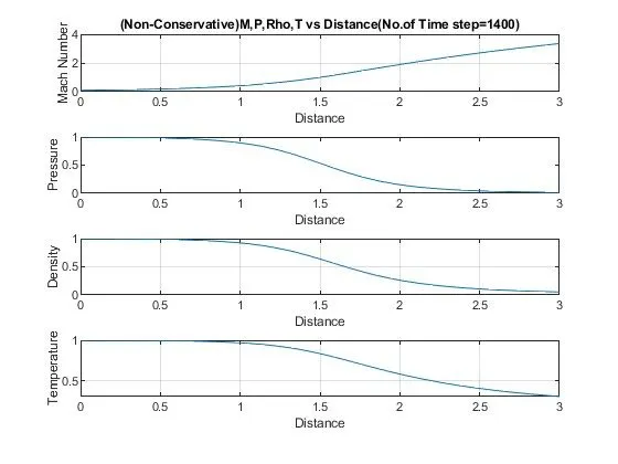
Plot for Variation of temperature ,Density, Pressure & Mach Number (Conservative Form) vs No of Timestep:

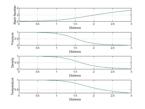
2.Steady-state distribution of primitive variables inside the nozzle:

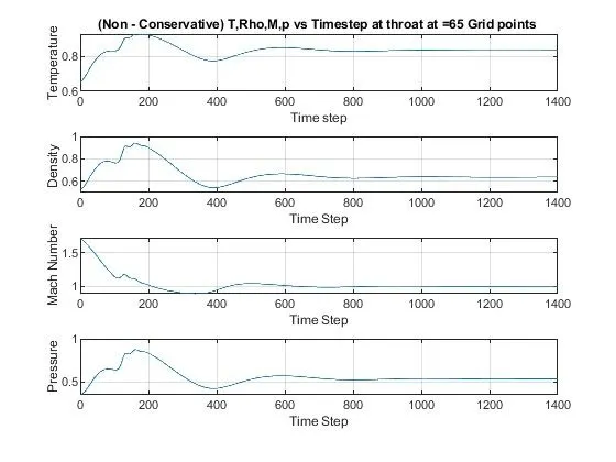
Plot for Variation of temperature ,Density, Pressure & Mach Number (Non-Conservative) at throat vs No of Timestep:

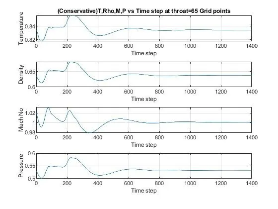
Plot for Variation of temperature ,Density, Pressure & Mach Number (Conservative) at throat vs No of Timestep:

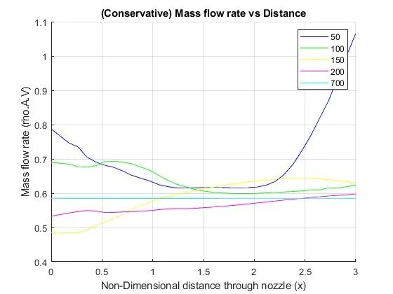
3) Variation of Mass flow rate distribution inside the nozzle at different time steps during the time-marching process

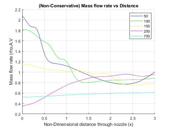
Plot for Variation of mass flow rate (Non-Conservative) vs Distance through Nozzle (x):

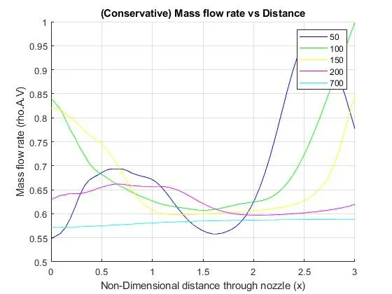
Plot for Variation of mass flow rate (Conservative) vs Distance through Nozzle (x):

4)Comparison of Normalized mass flow rate distributions of both forms

Plot for Variation of mass flow rate (Conservative) vs Distance through Nozzle (x):

For Grid Points = 65

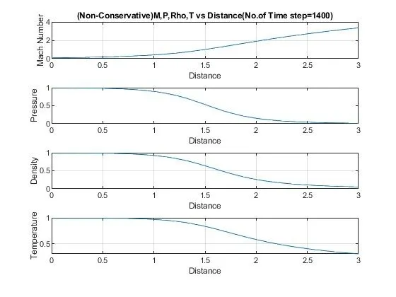
1.Time-wise variation of the primitive variables

Plot for Variation of temperature ,Density, Pressure & Mach Number (Non - Conservative form) vs No of Timestep:

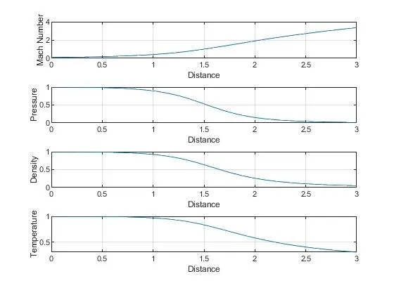
Plot for Variation of temperature ,Density, Pressure & Mach Number (Conservative Form) vs No of Timestep:

2.Steady-state distribution of primitive variables inside the nozzle:

Plot for Variation of temperature ,Density, Pressure & Mach Number (Non-Conservative) at throat vs No of Timestep:

Plot for Variation of temperature ,Density, Pressure & Mach Number (Conservative) at throat vs No of Timestep:

3) Variation of Mass flow rate distribution inside the nozzle at different time steps during the time-marching process

Plot for Variation of mass flow rate (Non-Conservative) vs Distance through Nozzle (x):

Plot for Variation of mass flow rate (Conservative) vs Distance through Nozzle (x):

4)Comparison of Normalized mass flow rate distributions of both forms

Plot for Variation of mass flow rate (Conservative) vs Distance through Nozzle (x):

Week 7 - Simulation of a 1D Supersonic nozzle flow simulation using Macormack Method

Ship work like this
in your own course.

Talk to a career counsellor

Ship work like thisin your own course.

Talk to a career counsellor

Ship work like this
in your own course.