Week 7 - Simulation of a 1D Supersonic nozzle flow simulation using Macormack Method
AIM
To simulate the isentropic flow through a quasi 1D subsonic-supersonic nozzle and derive both the conservation and non-conservation forms of the governing equations and sovle them using the MacCormack's technique. Also to determine the steady-state temperature distribution for the flow-field variables and investigate the difference between the two forms of governing equations by comparing their solutions.
INTRODUCTION
In this flow problem, we consider the steady, isentropic flow through a convergent-divergent nozzle as depictated in the below figure. The flow at the inlet to the nozzle comes from a reservoir where the pressure and temperature are denoted by p0 , and To, respectively. The cross-sectional area of the reservoir is large, and hence the velocity is very small. Thus, Po and T0 are the stagnation values or total pressure and total temperature, respectively. The flow expands isentropically to supersonic speeds at the nozzle exit, where the exit pressure, temperature, velocity, and Mach number are denoted by Pe, Te, Ve, and Me, respectlvely. The flow is locally subsonic in the convergent section of the nozzle, sonic at the throat (minimum area), and supersonic at the divergent section. The sonic flow (M = 1) at the throat means that the local velocity at this location is equal to the local speed of sound. Using an asterisk to denote sonic flow values, we have at the throat V = V* = a*. Similarly, the sonic flow values of pressure and temperature are denoted by p* and T*, respectively. The area of the sonic throat is denoted by A*.
We assume that at a given section, where the cross-sectional area is A, the flow properties are uniform across that section. Hence, although the area of the nozzle changes as a function of distance along the nozzle, x, and therefore in reality the flow field is two-dimensional, we make the assumption that the flow properties-vary only with x; this is tantamount to assuming uniform flow properties across any given cross section. Such flow is defined as quasi-one-dimensional flow.
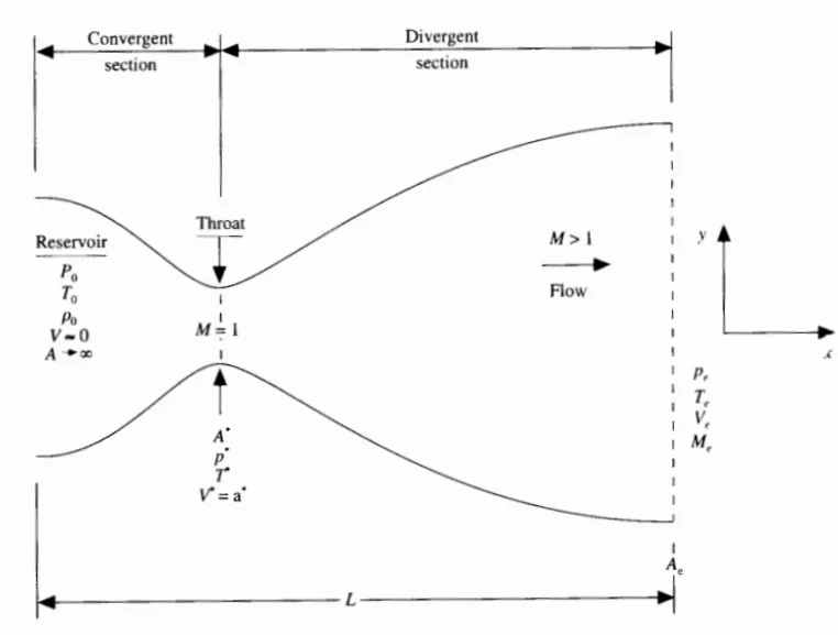
We now set up a time-marching finite difference solution for the above quasi-one-dimensional nozzle flow using Maccormack's technique which is an explicit method, both second order accurate in time and space and which is exclusively used for compressible flows.
THE SET UP
We divide this section into three steps -
- We derive both the conservation and non-conservation forms of the governing equations because the equations for an inviscid flow (Euler's equations) cannot be used directly for our problem as we have assumed the flow to be quasi-static and if we directly write the Euler's equations for 1-D flow, our assumption twists the real physics of the flow.
- Find a solution to these equations using the Maccormack's technique and also come up with determination of time step size and boundary conditions.
- Finally write a code and visualize our results through various appropriate plots.
1. Governing partial differential equations for unsteady quasi one dimensional flow -
Continuity equation
Non-conservation form - `(∂( ρ A))/(∂t)+V (∂ ( ρ A))/(∂x) = − ρ A (∂V)/(∂ x)`
Conservation form - `(∂( ρ A ))/ (∂t)+ (∂ ( ρ A V ))/(∂x) = 0`
Momentum equation
Non-conservation form - `ρ (∂V)/(∂t) + ρV (∂V)/(∂x) = − R [ ρ(∂T)/(∂x) + T(∂ρ)/(∂x)]`
Conservation form - `(∂(ρAV))/(∂t) + (∂(ρAV^2))/(∂x) = − A(∂P)/(∂x)`
Energy equation
Non-conservation form - `ρ(∂e)/(∂t) + ρV(∂e)/(∂x) = − P(∂V)/(∂x) − PV(∂(lnA))/(∂x)`
Conservation form - `(∂( ρ e A ))/(∂t) + (∂( ρ e V A ))/(∂x) = − P(∂( A V ))/(∂x)`
When we look at the continuity, momentum, and energy equations. We can see that; there are three equations and four unknowns/variables (ρ,V,P,T">ρ,V,P,T). The pressure (P">P) can be eliminated from these equations by using the equation of state: P = ρRT
The flow-field variables are frequently expressed in terms of nondimensional variables such as follows -
Dimensionless Temperature: T′=T/T0
Dimensionless Density: ρ′=ρ/ρ0
Dimensionless Length: x'=x/L
Dimensionless Velocity: V'=V/a0
Dimensionless Time: t'=t/(L/a0)
Dimensionless Area: A'=A/A*
Meshing -
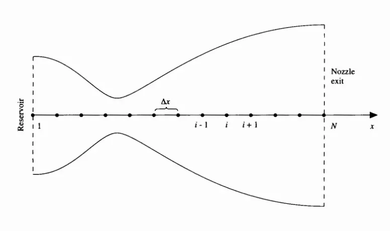
We divide the x axis along the nozzle into a finite number of discrete grid points. The first grid point, labeled point 1, is assumed to be in the reservoir. The points are evenly distributed along the x axis, with dx denoting the spacing between grid points. The last point, namely, that at the nozzle exit, is denoted by N; we have a total number of 31 grid points distributed along the axis. Point i is simply an arbitrary grid point, with points i - I and i + I as the adjacent points.
2. Solution to the governing equations using Maccormak's technique -
Non-conservation form - To implement a finite-difference solution to the above governing PDE's, we divide the x axis along the nozzle into a number of discrete grid points, as shown in the above figure. Here the first grid point, labeled point 1, is assumed to be in the reservoir. The points are evenly distributed along the x axis, with dx denoting the spacing between grid points. The last point, namely, that at the nozzle exit, is denoted by N; we have a total number of N grid points distributed along the axis. First, consider the predictor step.
Predictor step -



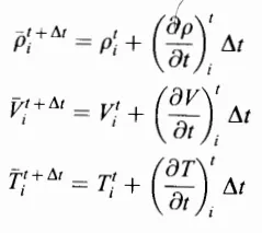
We next obtain predicted values of ρ, v, and T, denoted by barred quantities, from the below equations
Moving to the corrector step, we replace the spatial denvatlves with rearward differences, using the predicted (barred)
quantities as shown below
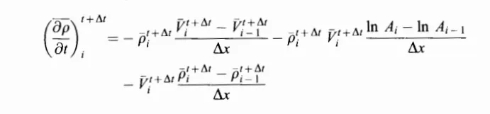

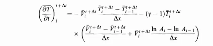
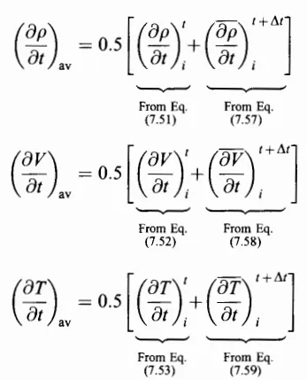
The average time derivatives are given by
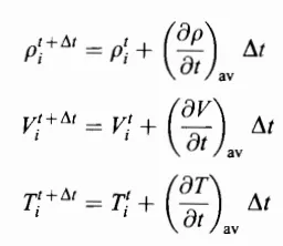
Finally, we have for the corrected values of the flow-field variables at time t + dt
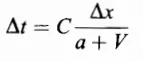
Calculation of time step size (dt) - Now the time step size is calculated for every grid point and for a particular time step, the minimum of the step size is considered. Also the step size is decided by the CFL criteria which disctates that the step size should be below a certain value for the solution to be stable. Here C is assumed to be 0.5 which is the Courant number.
Boundary conditions - At the subonic inflow boundary, we must stipulate the values of two dependent flow-field variables i.e., density and temperature, whereas the value of one other variable i.e., velocity, must be allowed to float. Similarly at supersonic outflow boundary, no flow-field variables which require their values to be stipulated at the supersonic outflow boundary; all variables must be allowed to float at this boundary.
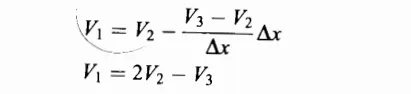
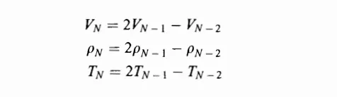
Initial conditions - In the present problem, we know that ρ and T decrease and V increases as the flow expands through the nozzle. Hence, we choose initial conditions that qualitatively behave in the same fashion.
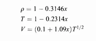
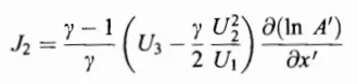
Conservation form - The equations for quasi-one dimensional flow are defined as the elements of the solution vector U, the flux vector F, and the source term J as follows.
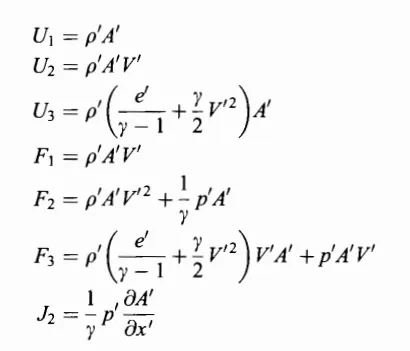
With these elements, the governing equations can be expressed as follows
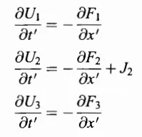
In the conservation form of the equations, the dependent variables (the variables for which we directly obtain numbers) are not the primitive variables and our numerical solution will give us numbers directly for U1 , U2 , and U3 in steps of time; this is why U is called the solutions vector. To obtain the primitive variables (p, V, T,p, etc.), we must decode the elements U1, U2, and U3 as follows. From the definitions of U1 , U2 , and U3 given above, we have
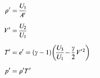
We note that the flux vector elements F1, F2, and F3 are couched in terms of the primitive variables . It has
been observed that when the computer program is written with F1, F2 and F3 expressed directly in terms of p', V', p', and e', instabilities develop during the course of the time-marching solution. For example, in the present example of quasi-one-dimensional, subsonic-supersonic, isentropic nozzle flow, instabilities develop in the subsonic section which finally cause the program to blow up after about 300 time steps. This behavior is an example of a lack of "purity" in the formulation of the governing equations in conservation form, a lack which eventually causes numerical problems. For this reason it is best to couch F1,F2,F3 directly in terms of U1, U2 and U3 and to avoid the use of primitive variables.

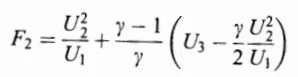
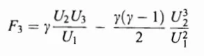
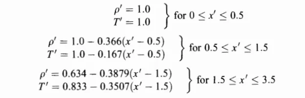
The boundary conditions and time step size calculation remain the same as discussed above for the non-conservative form. Only the initial conditions change and have been discussed below
CODE AND THE OUTPUT
clear
close all
clc

% Initial conditions
n=31;
L=3;
x=linspace(0,L,n);
dx=x(2)-x(1);

A= 1+2.2*(x-1.5).^2;

gamma=1.4;
nt=1400; %time-steps
C=0.5; %Courant number

% Calling function to solve the non-conservative form of the GE's
tic
[rho1,T1,V1,P1,M1,m1,rho_throat1,V_throat1,T_throat1,P_throat1,M_throat1,residual1]= non_conservative_func(x,dx,A,C,nt,gamma);
Time_taken_by_non_conservative_form=toc;


% Calling function to solve the conservative form of the GE's
tic
[rho2,V2,T2,P2,M2,m2,rho_throat2,V_throat2,T_throat2,M_throat2,P_throat2,residual2]= conservative_func(x,dx,A,C,gamma,nt);
Time_taken_by_conervative_form=toc;


% Plots for different flow parameters: Non-Conservative form
figure (1)
subplot (4,1,1)
plot (x,M1,'LineWidth',2)
grid on
grid minor;
ax=gca;
ax.FontSize=14;
ylim ([0,4.5])
yticks (0:1.5:4.5)
ylabel ('Mach number','FontSize',12,'FontWeight','bold')
title ('Steady-state distribution of primitive variables inside the nozzle: Non-Conservative Form ','FontSize',12,'FontWeight','Bold','color','b')

subplot (4,1,2)
plot (x,P1,'LineWidth',2)
grid on
grid minor
ax=gca;
ax.FontSize=14;
yticks (0:0.2:1);
ylabel ('Pressure ratio','FontSize',12,'FontWeight','bold')

subplot (4,1,3)
plot (x,rho1,'LineWidth',2)
grid on
grid minor
ax=gca;
ax.FontSize=14;
yticks (0:0.2:1)
ylabel ('Density ratio','FontSize',12,'FontWeight','bold')

subplot (4,1,4)
plot (x,T1,'LineWidth',2)
grid on
grid minor
ax=gca;
ax.FontSize=14;
ylim ([0,1])
yticks (0:0.2:1)
ylabel ('Temperature ratio','FontSize',12,'FontWeight','bold')
xlabel ('x/L','FontSize',12,'FontWeight','bold')

% Plots for different flow parameters: Conservative form
figure (2)
subplot (4,1,1)
plot (x,M2,'LineWidth',2)
grid on
grid minor;
ax=gca;
ax.FontSize=14;
ylim ([0,4.5])
yticks (0:1.5:4.5)
ylabel ('Mach number','FontSize',12,'FontWeight','bold')
title ('Steady-state distribution of primitive variables inside the nozzle: Conservative Form','FontSize',12,'FontWeight','Bold','color','b')

subplot (4,1,2)
plot (x,P2,'LineWidth',2)
grid on
grid minor
ax=gca;
ax.FontSize=14;
yticks (0:0.2:1);
ylabel ('Pressure ratio','FontSize',12,'FontWeight','bold')

subplot (4,1,3)
plot (x,rho2,'LineWidth',2)
grid on
grid minor
ax=gca;
ax.FontSize=14;
yticks (0:0.2:1)
ylabel ('Density ratio','FontSize',12,'FontWeight','bold')

subplot (4,1,4)
plot (x,T2,'LineWidth',2)
grid on
grid minor
ax=gca;
ax.FontSize=14;
ylim ([0,1])
yticks (0:0.2:1)
ylabel ('Temperature ratio','FontSize',12,'FontWeight','bold')
xlabel ('x/L','FontSize',12,'FontWeight','bold')

% Plots for different flow parameters at 'Throat Section': Non-conservative vs. Conservative form
figure (3)
subplot (4,1,1)
plot (1:nt,M_throat1,'LineWidth',2)
hold on
plot (1:nt,M_throat2,'LineWidth',2)
grid on
grid minor
ax=gca;
ax.FontSize=12;
yticks (0:0.2:2)
ylabel ('Mach Number','FontSize',15,'FontWeight','bold')
l_g_d=legend('Non-Conservative','Conservative');
l_g_d.FontSize=15;
title ('Time-wise variation of the primitive variables','FontSize',15,'FontWeight','bold','color','b')

subplot (4,1,2)
plot (1:nt,P_throat1,'LineWidth',2)
hold on
plot (1:nt,P_throat2,'LineWidth',2)
grid on
grid minor
ax=gca;
ax.FontSize=12;
yticks (0:0.2:1)
ylabel ('P/P_0','FontSize',15,'FontWeight','bold')
l_g_d=legend('Non-Conservative','Conservative');
l_g_d.FontSize=15;

subplot (4,1,3)
plot (1:nt,rho_throat1,'LineWidth',2)
hold on
plot (1:nt,rho_throat2,'LineWidth',2)
grid on
grid minor
ax=gca;
ax.FontSize=12;
yticks (0:0.2:1)
ylabel ('rho/rho_0','FontSize',15,'FontWeight','bold')
l_g_d=legend('Non-Conservative','Conservative');
l_g_d.FontSize=15;

subplot (4,1,4)
plot (1:nt,T_throat1,'LineWidth',2)
hold on
plot (1:nt,T_throat2,'LineWidth',2)
grid on
grid minor
ax=gca;
ax.FontSize=12;
yticks (0:0.2:1)
ylabel ('T/T_0','FontSize',15,'FontWeight','bold')
xlabel ('Time Steps','FontSize',15,'FontWeight','bold')
l_g_d=legend('Non-Conservative','Conservative');
l_g_d.FontSize=15;

% Plot for Mass Flow Rate variation: Non-conservative form
figure (4)
plot (x,m1(50,:),'-*','LineWidth',2)
hold on
grid on
grid minor
plot (x,m1(100,:),'-x','LineWidth',2)
hold on
plot (x,m1(150,:),'-d','LineWidth',2)
hold on
plot (x,m1(200,:),'-p','LineWidth',2)
hold on
plot (x,m1(500,:),'-o','LineWidth',2)
hold on
plot (x,m1(700,:),'-s','LineWidth',2)
hold on
plot (x,m1(1400,:),'--','LineWidth',2)
xlabel ('x/L','FontSize',15,'FontWeight','bold')
ylabel ('rhoAV/rho_0A^*a_0','FontSize',15,'FontWeight','bold')
l_g_d=legend ('50 Deltat','100 Deltat','150 Deltat','200 Deltat','500 Deltat','700 Deltat','1400 Deltat');
l_g_d.FontSize=14;
title ('Variation of Mass flow rate distribution at different time steps: Non-conservative Form','FontSize',12,'FontWeight','bold','color','b')

% Plot for Mass Flow Rate variation: Conservative form
figure (5)
plot (x,m2(50,:),'-*','LineWidth',2)
hold on
grid on
grid minor
plot (x,m2(100,:),'-x','LineWidth',2)
hold on
plot (x,m2(150,:),'-d','LineWidth',2)
hold on
plot (x,m2(200,:),'-p','LineWidth',2)
hold on
plot (x,m2(500,:),'-o','LineWidth',2)
hold on
plot (x,m2(700,:),'--','LineWidth',2)
xlabel ('x/L','FontSize',15,'FontWeight','bold')
ylabel ('rhoAV/rho_0A^*a_0','FontSize',15,'FontWeight','bold')
l_g_d=legend ('50 Deltat','100 Deltat','150 Deltat','200 Deltat','500 Deltat','700 Deltat');
l_g_d.FontSize=14;
title ('Variation of Mass flow rate distribution at different time steps: Conservative Form','FontSize',12,'FontWeight','bold','color','b')

% Plot for variation of Non-dimensional Mass Flow Rate-Steady State: Non-conservative vs. Conservative form vs. Exact Solution
figure (6)
plot (x,0.579*ones(length(x),1),'--','Linewidth',2)
hold on
grid on
grid minor
plot (x,m1(end,:),'LineWidth',2)
hold on
plot (x,m2(end,:),'LineWidth',2)
ax=gca;
ax.FontSize=12;
xlabel ('x/L','FontSize',15,'FontWeight','bold')
ylabel ('rhoAV/rho_0A^*a_0','FontSize',15,'FontWeight','bold')
legend ('Exact','Non-conservative','Conservative','FontSize',15)
title ('Comparison of Normalized mass flow rate distributions of both forms','FontSize',15,'FontWeight','bold','color','b')

%% Function for non-conservation form of GE's

function [rho1,T1,V1,P1,M1,m1,rho_throat1,V_throat1,T_throat1,P_throat1,M_throat1,residual1]= non_conservative_func(x,dx,A,C,nt,gamma)


% Density
rho_at_t_0=1-0.314*x;

% Temperature
T_at_t_0=1-0.2314*x;

% Velocity
V_at_t_0=(0.1+1.09*x).*T_at_t_0.^(0.5);

rho1=rho_at_t_0;
T1=T_at_t_0;
V1=V_at_t_0;

% Mass flow rate
m1=zeros(nt,length(x));

% Defining area at throat
throat=find(A==1);

% Initial condition of variables at the throat section:
rho_throat1=zeros(nt,1); %Density @ throat
T_throat1=rho_throat1; %Temperature @ throat
V_throat1=T_throat1; %Velocity @ throat
P_throat1=V_throat1; %Pressure @ throat
M_throat1=P_throat1; %Mach number @ throat

residual1=zeros(nt,3);

% Using MacCormack Method:
% Time-Loop
for k=1:nt

    % Creating a copy of old values
    rho_old=rho1;
    T_old=T1;
    V_old=V1;

    % Stability criterion (CFL condition)
    % Time-step (dt)
    dt=min(C*dx./(T1.^0.5+V1));

    % Predictor-Step
    % Space-Loop
    for i=2:length(x)-1

        % Discretizing using forward difference scheme for spatial derivatives
        dVdx=(V1(i+1)-V1(i))/dx;
        dlogAdx=(log(A(i+1))-log(A(i)))/dx;
        drhodx=(rho1(i+1)-rho1(i))/dx;
        dTdx=(T1(i+1)-T1(i))/dx;

        % Continuity equation
        drho_dt_p(i)=-rho1(i)*dVdx-rho1(i)*V1(i)*dlogAdx-V1(i)*drhodx;

        % X-Momentum equation
        dV_dt_p(i)=-V1(i)*dVdx-(1/gamma)*(dTdx+(T1(i)/rho1(i))*drhodx);

        % Energy equation
        dT_dt_p(i)=-V1(i)*dTdx-(gamma-1)*T1(i)*(dVdx+V1(i)*dlogAdx);

        % Interim Solution update
        rho1(i)=rho1(i)+drho_dt_p(i)*dt;
        V1(i)=V1(i)+dV_dt_p(i)*dt;
        T1(i)=T1(i)+dT_dt_p(i)*dt;
    end % end of space loop (Predictor-step)

    % Corrector-Step
    % Space-Loop
    for i=2:length(x)-1

        % Discretizing using backward difference scheme for spatial derivatives
        dVdx=(V1(i)-V1(i-1))/dx;
        dlogAdx=(log(A(i))-log(A(i-1)))/dx;
        drhodx=(rho1(i)-rho1(i-1))/dx;
        dTdx=(T1(i)-T1(i-1))/dx;

        % Continuity equation
        drho_dt_c(i)=-rho1(i)*dVdx-rho1(i)*V1(i)*dlogAdx-V1(i)*drhodx;

        % X-Momentum equation
        dV_dt_c(i)=-V1(i)*dVdx-(1/gamma)*(dTdx+(T1(i)/rho1(i))*drhodx);

        % Energy equation
        dT_dt_c(i)=-V1(i)*dTdx-(gamma-1)*T1(i)*(dVdx+V1(i)*dlogAdx);

    end % end of space loop (Corrector-step)

    % Computing the average time derivative
    drho_dt=0.5*(drho_dt_p+drho_dt_c);
    dV_dt=0.5*(dV_dt_p+dV_dt_c);
    dT_dt=0.5*(dT_dt_p+dT_dt_c);

    residual1(k,1)=max(abs(drho_dt));
    residual1(k,2)=max(abs(dV_dt));
    residual1(k,3)=max(abs(dT_dt));

    % Final solution update
    for j=2:length(x)-1
        rho1(j)=rho_old(j)+(drho_dt(j)*dt);
        V1(j)=V_old(j)+(dV_dt(j)*dt);
        T1(j)=T_old(j)+(dT_dt(j)*dt);
    end

% Applying Boundary Conditions:-
% Subsonic Inflow Boundary:
V1(1)=2*V1(2)-V1(3); % Velocity at the inlet

% Supersonic Outflow Boundary:
V1(end)=2*V1(end-1)-V1(end-2); % Velocity at outlet
rho1(end)=2*rho1(end-1)-rho1(end-2); % Density at outlet
T1(end)=2*T1(end-1)-T1(end-2); % Temperature at outlet

% Mass flow rate
m1(k,:)=rho1.*A.*V1;

% Pressure (P)
P1=rho1.*T1;

% Mach number
M1=V1./(T1.^0.5);

% Values at throat:-
rho_throat1(k)=rho1(throat);
M_throat1(k)=M1(throat);
P_throat1(k)=P1(throat);
T_throat1(k)=T1(throat);
V_throat1(k)=V1(throat);
end
end

%% Function for conservation form of GE's


function [rho2,V2,T2,P2,M2,m2,rho_throat2,V_throat2,T_throat2,M_throat2,P_throat2,residual2] = conservative_func(x,dx,A,C,gamma,nt)

% Initial Conditions (at time, t=0)
rho_at_t_0=zeros(1,length(x));
T_at_t_0=rho_at_t_0;
V_at_t_0=T_at_t_0;

for i=1:length(x)
    if x(i)>=0 && x(i)<0.5
        rho_at_t_0(i)=1;
        T_at_t_0(i)=1;

    elseif x(i)>=0.5 && x(i)<1.5
            rho_at_t_0(i)=1-0.366*(x(i)-0.5);
            T_at_t_0(i)=1-0.167*(x(i)-0.5);

    elseif x(i)>=1.5 && x(i)<=3.5
                rho_at_t_0(i)=0.634-0.3879*(x(i)-1.5);
                T_at_t_0(i)=0.833-0.3507*(x(i)-1.5);

    end
    V_at_t_0(i)=0.59/(rho_at_t_0(i)*A(i));
end

rho2=rho_at_t_0;
T2=T_at_t_0;
V2=V_at_t_0;

% Mass flow rate
m2=zeros(nt,length(x));


% Initial Conditions for the solution vectors (U)
U1=rho2.*A;
U2=rho2.*A.*V2;
U3=rho2.*A.*((T2./(gamma-1))+(gamma/2).*(V2.^2));

% Defining area at throat
throat=find(A==1);

% Initial condition of variables at the throat section:
rho_throat2=zeros(nt,1); %Density @ throat
T_throat2=rho_throat2; %Temperature @ throat
V_throat2=T_throat2; %Velocity @ throat
P_throat2=V_throat2; %Pressure @ throat
M_throat2=P_throat2; %Mach number @ throat

residual2=zeros(nt,3);

% Using MacCormack method
% Time-Loop
 for k=1:nt

     % Creating a copy of Old Values
     U1_old=U1;
     U2_old=U2;
     U3_old=U3;

     % Stability criterion (CFL condition)
     % Time-step (dt)
     dt=min(C*dx./(T2.^0.5+V2));

     % Initial Conditions for flux vectors (F)
     F1=U2;
     F2=(U2.^2)./U1+((gamma-1)/gamma)*(U3-0.5*gamma*(U2.^2)./U1);
     F3=gamma*U2.*U3./U1-0.5*gamma*(gamma-1)*(U2.^3)./(U1.^2);

     % Predictor-Step
     % Space-Loop
     for i=2:length(x)-1
         % Discretizing using forward difference scheme for spatial derivatives
         % Source Vector
         J2=(1/gamma)*rho2(i)*T2(i)*((A(i+1)-A(i))/dx);

         % Continuity Equation
         dU1_dt_p(i)=-(F1(i+1)-F1(i))/dx;

         % Momentum Equation
         dU2_dt_p(i)=-(F2(i+1)-F2(i))/dx+J2;

         % Energy Equation
         dU3_dt_p(i)=-(F3(i+1)-F3(i))/dx;

         % Interim Solution Update

         U1(i)=U1(i)+dU1_dt_p(i)*dt;
         U2(i)=U2(i)+dU2_dt_p(i)*dt;
         U3(i)=U3(i)+dU3_dt_p(i)*dt;

     end

     % Obtaining the Primitive variables form our solution vector (U1,U2,U3):-
     rho2=U1./A;
     V2=U2./U1;
     T2=(gamma-1)*((U3./U1)-((gamma/2)*(V2.^2)));

     % Updating Flux Vectors
     F1=U2;
     F2=((U2.^2)./U1)+(((gamma-1)/gamma)*(U3-((gamma/2)*(U2.^2./U1))));
     F3=((gamma.*U2.*U3)./U1)-((gamma*(gamma-1))/2)*(U2.^3)./(U1.^2);

     % Corrector-Step
     % Space-Loop
     for i=2:length(x)-1
         % Discretizing using backward difference scheme for spatial derivatives
         % Source Vector
         J2=(1/gamma)*rho2(i)*T2(i)*((A(i)-A(i-1))/dx);

         % Continuity Equation
         dU1_dt_c(i)=-(F1(i)-F1(i-1))/dx;

         % Momentum Equation
         dU2_dt_c(i)=-(F2(i)-F2(i-1))/dx+J2;

         % Energy Equation
         dU3_dt_c(i)=-(F3(i)-F3(i-1))/dx;

     end

     % Computing the average time derivative
     dU1_dt=0.5*(dU1_dt_p+dU1_dt_c);
     dU2_dt=0.5*(dU2_dt_p+dU2_dt_c);
     dU3_dt=0.5*(dU3_dt_p+dU3_dt_c);

     residual2(k,1)=max(abs(dU1_dt));
     residual2(k,2)=max(abs(dU2_dt));
     residual2(k,3)=max(abs(dU3_dt));

     % Final Solution Update
     for j=2:length(x)-1
         U1(j)=U1_old(j)+dU1_dt(j)*dt;
         U2(j)=U2_old(j)+dU2_dt(j)*dt;
         U3(j)=U3_old(j)+dU3_dt(j)*dt;
     end

% Subsonic Inflow Boundary
U1(1)=rho2(1)*A(1);
U2(1)=2*U2(2)-U2(3);
U3(1)=U1(1)*((T2(1)/(gamma-1))+0.5*gamma*V2(1)^2);

% Supersonic Outflow Boundary
U1(end)=2*U1(end-1)-U1(end-2);
U2(end)=2*U2(end-1)-U2(end-2);
U3(end)=2*U3(end-1)-U3(end-2);

% Final values of different variables:
rho2=U1./A; %Density
V2=U2./U1; %Velocity
T2=(gamma-1)*((U3./U1)-0.5*gamma*V2.^2); %Temperature
M2=V2./(T2.^0.5); %Mach number
P2=rho2.*T2; %Pressure
m2(k,:)=rho2.*A.*V2; %Mass flow rate

rho_throat2(k)=rho2(throat);
V_throat2(k)=V2(throat);
T_throat2(k)=T2(throat);
P_throat2(k)=P2(throat);
M_throat2(k)=M2(throat);

end
end
a. Steady-state distribution of primitive variables inside the nozzle
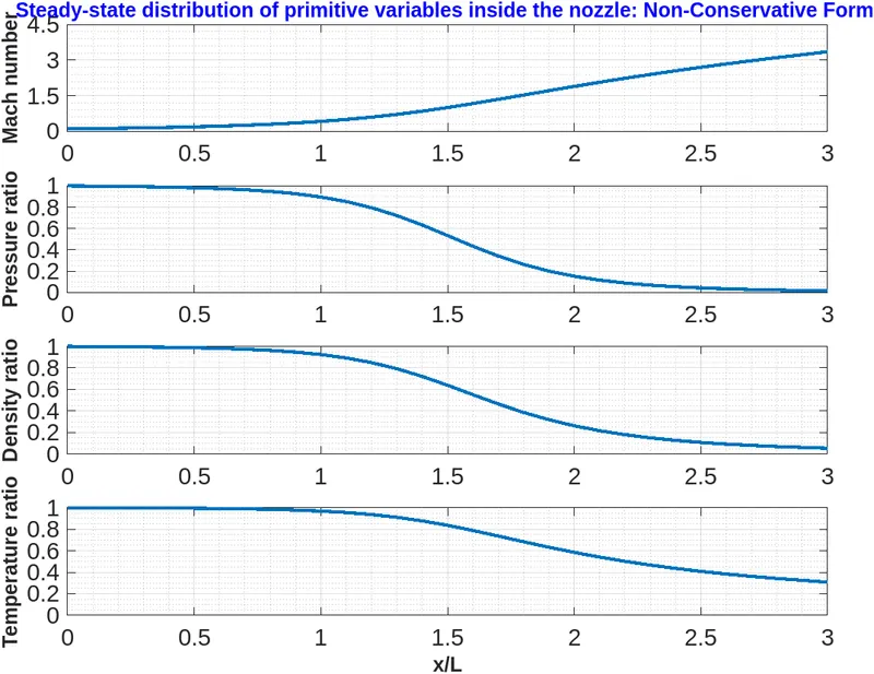
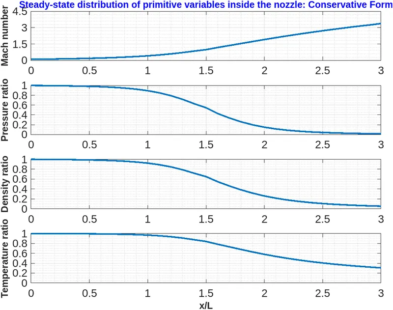
From the above plots we can see that, as the Mach number increases the primitive variables keep decreasing after the sonic region (Mach=1) till the exit of the nozzle. The steady-state results obtained from the time-marching solution for the governing equations in non-conservative form and conservative form are essentially the same but with a few slight, but notable differences.
b. Time-wise variation of the primitive variables considering throat section
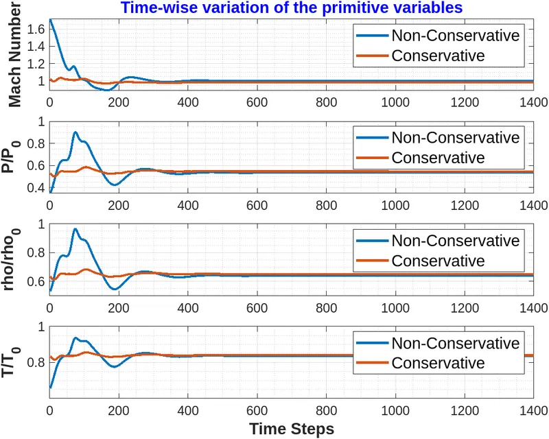
The above plots conclude that the values obtained for the primitive variables at the throat using conservation form converge faster than the non-conservation form.
c. Variation of Mass flow rate distribution inside the nozzle at different time steps during the time-marching process
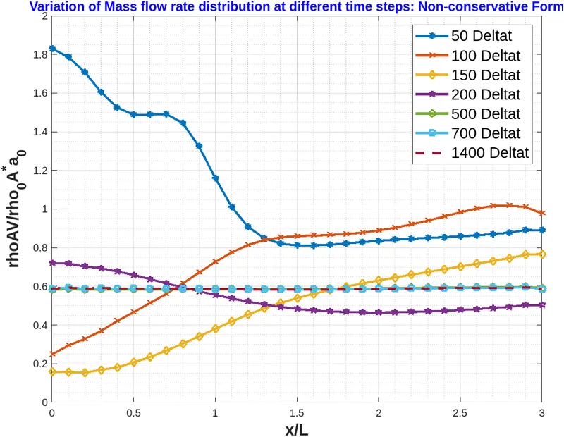
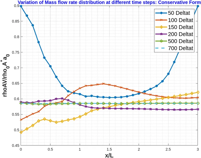
Here, the nondimensional mass flow rate is plotted as a function of nondimensional distance through the nozzle. Six different curves are shown, each for a different time during the course of the time-marching procedure. For the non-conservative form, we observe that after 500-time steps the mass flow is moving toward the steady-state value and at 700-time steps the mass flow distribution is a straight, horizontal line across the graph. This says that the mass flow has converged to a constant, steady-state value throughout the nozzle. For the conservative form, the mass flow rate at 500-time steps starts showing consistency, and after 700-time steps it is almost equal to a constant value. Moreover, it is quite close to the exact analytical value of 0.579.
d. Comparison of Normalized mass flow rate distributions of both forms
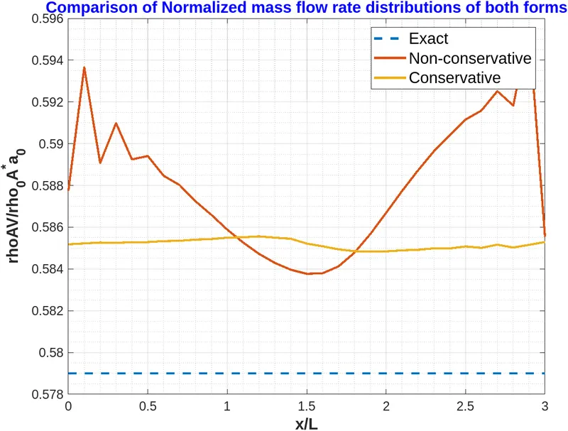
In the above plot, we compare the steady-state variations of mass flow obtained with the non-conservative and conservative forms of the governing equations and we see that the steady-state mass flow distribution predicted by the conservative form of the equations is much more satisfactory than that obtained from the non-conservative form, on two accounts:
- The conservative form gives a distribution i.e. much closer to being a constant. In contrast, the non-conservative results have a sizeable variation, with some spurious oscillations at both the inflow and outflow boundary.
- The steady-state mass flow results obtained with the conservative form are, on the whole, much closer to the exact analytical solution.
Grid independence test at the throat section - To answer the question do our calculations show grid independency, the grid spacing was reduced and a total of 61 grid points were created to perform this study. It was found that although the number of grid points were doubled from 31 to 61, the numerical solution improved only marginally. The same was true for all locations within the nozzle (As per the reference book). In other words, the two steady-state numerical solutions were essentially the same, and therefore we can conclude that our original calculations using 31 grid points is essentially grid-independent.
Note - The calculations shown below were performed using a seperate code and to avoid the lengthiness of the code, the results obtained are directly been tabulated.
| Density ratio | Temperature ratio | Pressure ratio | Mach number | |
| 31 grid points | 0.639 | 0.836 | 0.534 | 0.999 |
| 61 grid points | 0.638 | 0.835 | 0.533 | 1.000 |
CONCLUSION
- There is no clear superiority of either form in terms of accuracy of the results. The nonconservation form seems to produce slightly more accurate results for the primitive variables, and the conservation form seems to produce slightly more accurate results for the flux variables. The results in either case are certainly satisfactory.
- The conservation form yields a better mass flow distribution. The conservation form simply does a better job of conserving mass.
- The nonconservation form leads to smaller residuals. The amount by which the residuals decay is often used as an index of "quality" of the numerical algorithm. In this sense, the nonconservation form does a better job.
- Comparing the amount of calculational effort to achieve a solution, we note that the solution of the conservation form requires marginally more work. Most of this is due to the need to decode the primitive variables from the flux variables; such decoding is not necessary when we are solving the nonconservation form.