Week 4 - CHT Analysis on Exhaust port

                                                                                            AIM

    To simulate the flow inside an exhaust manifold and calculate the heat trasnfer coefficient numerically and then compare the simulation results with analytical results. Also to perform grid independence study to check the temperature and velocity contour plots for the default mesh and the refined mesh.

                                                                                 INTRODUCTION 

    Conjugate heat transfer (CHT) analysis is an analysis performed to analyze the heat transfer between solids and fluids. As we know that the mode of heat transfer in solids is conduction and in fluids it is either due to free or forced convection, it becomes necessary to study the behaviour of the fluids so as to understand various parameters like temperature, pressure, velocity, etc.

    A classic example of CHT is the transfer of heat from the heated spoon to the atmosphere until thermal equilibrium is reached. Here, the heat first conducts through the spoon to the top surface and then through natural convection it is transfered to the atmosphere. Using a proper mesh size, we can simulate the flow of heat and thus study various parameters like temperature, velocity, etc. 

    In the current project, CHT analysis is performed on exhaust manifold using ANSYS Fluent. Two different meshes are used for the analysis: 

1. Baseline mesh of 150 mm which generated 1.38 lakhs of elements.
2. Refined mesh of 20 mm which generated 2.8 lakhs of elements (excluding the inflation layers).

    The last step is to obtain the results from the simulation and compare the values with analytical results for the above two cases.

                                                                         PREPARING THE GEOMETRY

    After importing the given model in the Spaceclaim, we first extract the internal volume and then share the geometry so that there will a relation maintained between the the various geometries and this would help in meshing.

                                                                                 MESHING

Case 1 : Baseline mesh

• Base Mesh size - 150 mm
• Edge sizing - 36 number of divisions
• y+ value - 5 
• First cell height - 0.6 mm
• Number of inflation layers - 10
• Total boundary layer thickness - 14.5 mm

Case 2 : Refined mesh

• Base Mesh size - 20 mm
• Edge sizing - 36 number of divisions
• y+ value - 2
• First cell height - 0.22 mm
• Number of inflation layers - 10
• Total boundary layer thickness - 5.8 mm

 

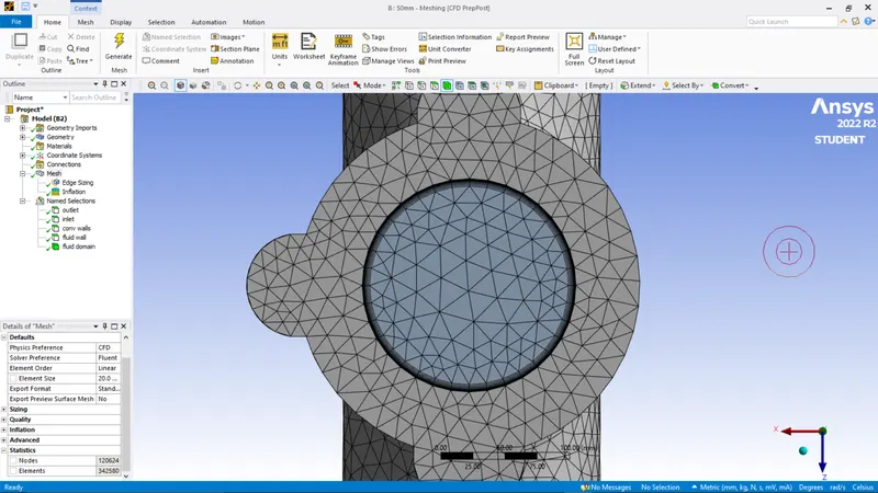
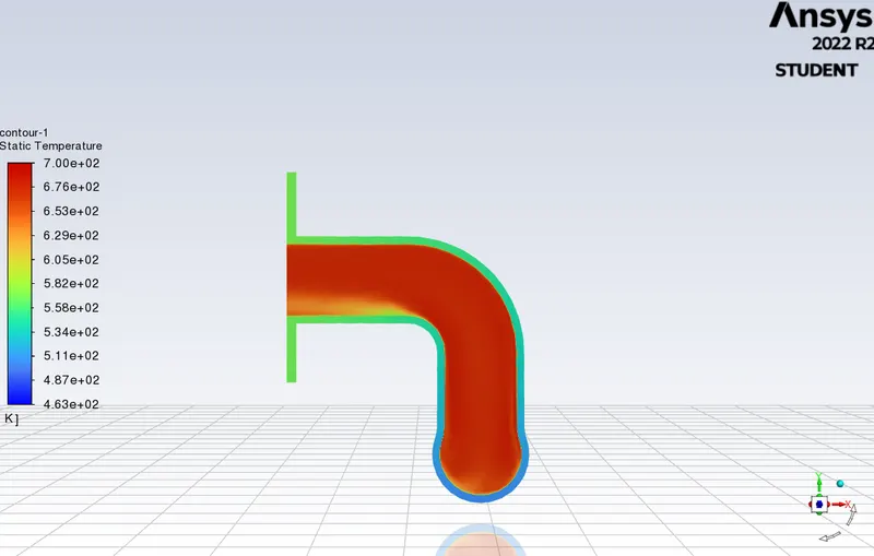
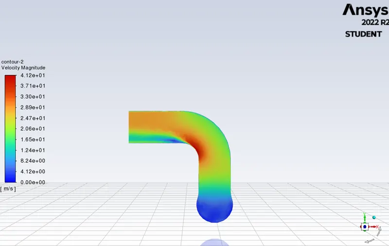
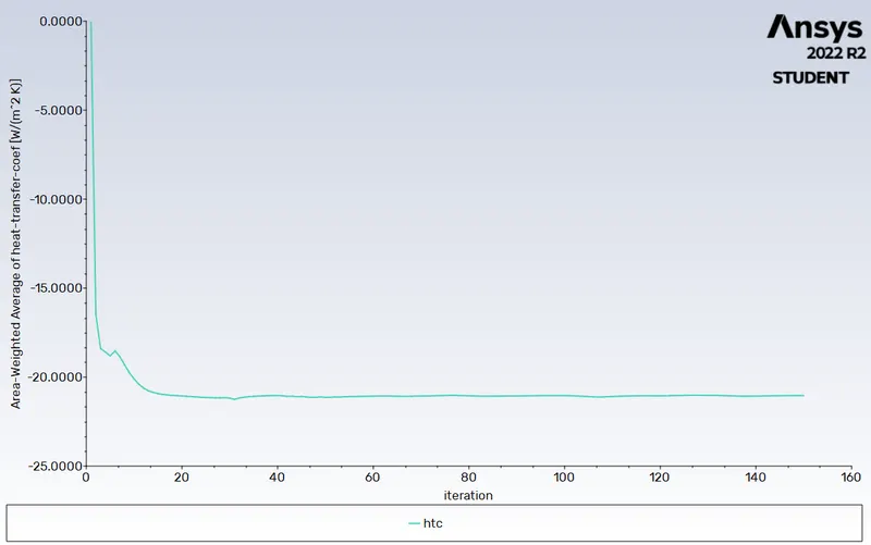
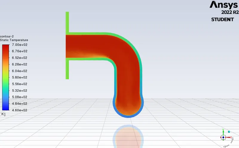
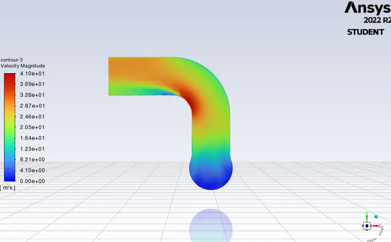
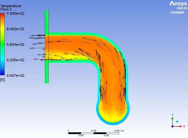
    Since there is transfer of heat at the interface of solid and fluid surfaces, we use k-epsilon turbulence model so properly capture the fluid parameters at the boundary. By reducing the y+ value from 5 to 2, one can easily visualize that more clear temperature and velocity gradients are observed as we refine the mesh although there is not much difference in the value of HTC whic has been discussed in the later stages.

                                                                       SOLVING APPROACH

    For both baseline mesh and refined mesh, the three dimensional Navier-Stokes equations are solved using a steady state pressure-based solver. For modeling turbulence the standard k-epsilon model is employed. 

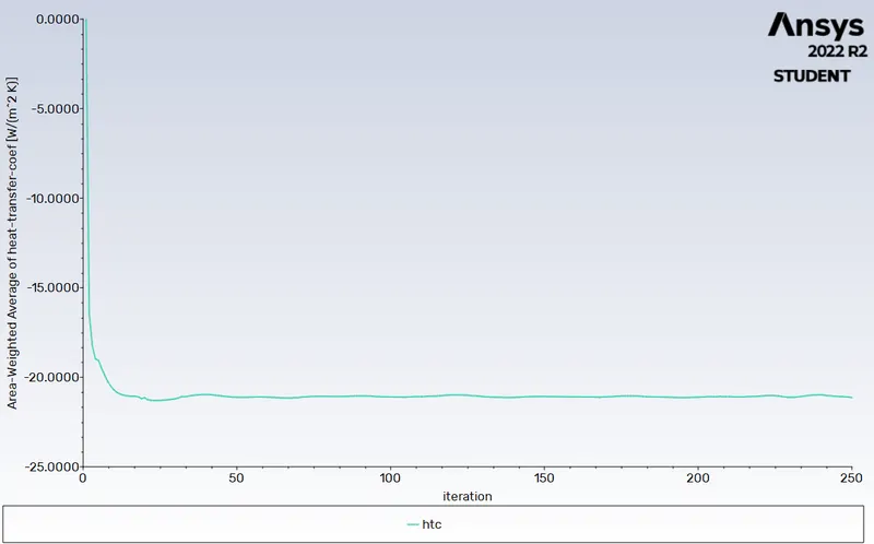
    The solution is initialized using a hybrid initialization scheme and similar boundary conditions are applied for both the cases. For both the cases the solver is run for 150 iterations since it is sufficient enough to get the converged solution. Temperature and velocity contours are plotted for both the cases.

                                                                              RESULTS

Case 1:

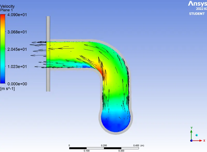
HTC,Velocity and temperature contours

Case 2:

Heat transfer coefficient (h) in W/m2.K	Baseline mesh	Refined mesh
Analytical	15.7	16.5
Numerical	21.015	21.05

    To check if the HTC predictions are right, we need to conduct experiments and then verify numerical reults with these experimental reults. But since conducting the experiments is time consuming and expensive and we have the analytic equations which are in algebraic form, we can compare the numerical values with the analytical values and thus validate our results.

Analytic results - To calculate the HTC for turbulent flow in a tube, we have the following equations,

First we calculate the Reynold's number using the following fluid parameters

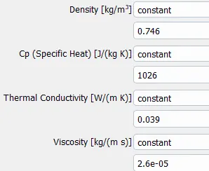 We get Re = 22954 which is greater than 10,000 and hence we use the following equation for the fluid being heated,

Nusselt number (Nu) = 0.023(Re)^0.8(Pr)^0.4       (All the properties are at 200 K)

                               = 60.5

                   HTC (h) = (Nu*k) / L 

                               = 15.7

                                                                               CONCLUSION

• Refined mesh generates smooth contour plots near the wall due to the presence of lower y+ values and hence the lower first cell height.
• At the tube bend, the fluid parameters are better solved for the refined mesh.

The factors on which the accuracy of the prediction depend on are as follows :

• Turbulence models - Appropriate mathematical models should be used to capture the various parameters correctly that is, for no-slip conditions use k-epsilon model and vice versa.
• Mesh size - Use refined mesh where the flow features are to be captured.
• Initial and boundary conditions - Use proper initialization method and appropriate BC at proper walls.
• Solvers - Use density based solvers for hypersonic flows or else pressure based solvers.