Week 7 - Simulation of a 1D Supersonic nozzle flow simulation using Macormack Method
OBJECTIVE :
To simulate the isentropic flow through a quasi 1D subsonic-supersonic nozzle.
CONDITIONING FOR THE OBJECTIVE GIVEN ;
- You will derive both the conservation and non-conservation forms of the governing equations and sovle them using the MacCormack's technique. You need to determine the steady-state temperature distribution for the flow-field variables and investigate the difference between the two forms of governing equations by comparing their solutions.
You need to show the following plots inside your report
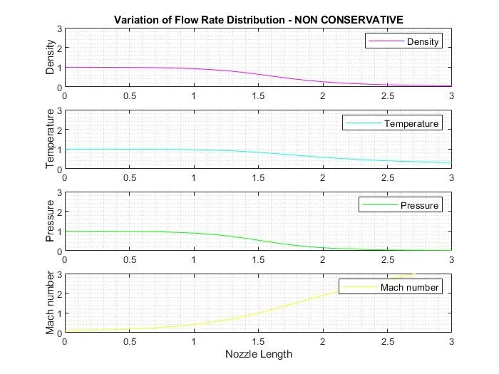
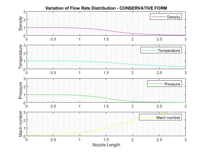
1. Steady-state distribution of primitive variables inside the nozzle
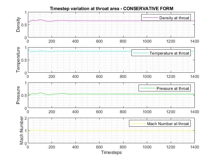
2. Time-wise variation of the primitive variables
3. Variation of Mass flow rate distribution inside the nozzle at different time steps during the time-marching process
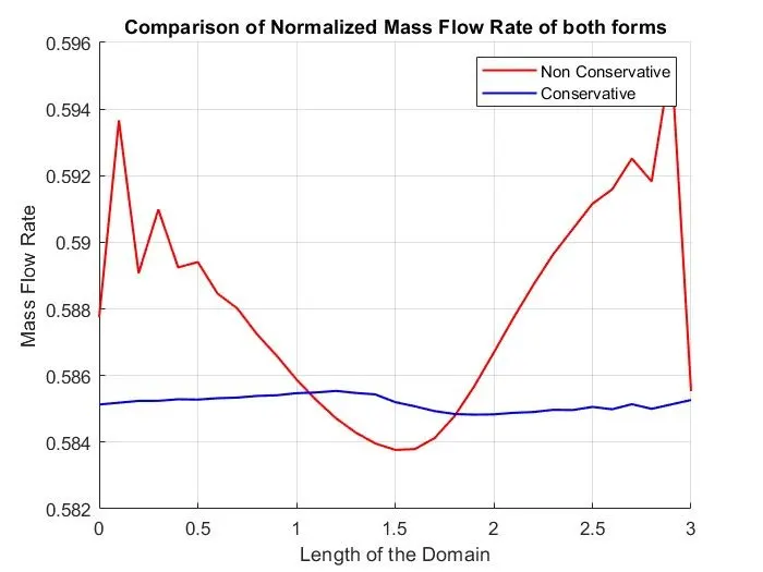
4. Comparison of Normalized mass flow rate distributions of both forms
EXPECTED RESULTS
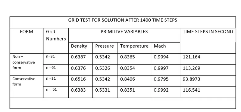
- Perform a grid independence test on the solution and expain all your findings.
- The code must be modular. You need to write separate functions to solve both forms.
- Discuss all the plots you are providing with observed inferences.
THEORY;
The system is considered as 1-D quasi supersonic nozzle performing in a steady state . The objective of the problem is to perform a simulation for this nozzle for finding the flow rates, primitive variables inside the nozzle flowing from convergent section to the divergent part which then undergoes change in quantities by surpassing the Throat section of the nozzle.
The simulation is done for both Conservative and Non - conservative form of the governing equation performing in the nozzle.
The nozzle is set to have the simulation right after the reservoir section as the area here tends to a very large section and the veloci is dropped contrastly. The simulation is done by the following steps
- meshing
- discritization
- solution part
The solution part is followed using Macormak method which involves
- PREDICTOR METHOD
- INTERMEDIATE SOLUTION UPDATE
- CORRECTOR METHOD
- AVERAGING (PREDICTOR AND CORRECTOR STEPS)
- FINAL TIME STEP UPDATE
The Macormak method is used as the governing partial derivatives head to a explicit time marchig solution , So the basic approach for this 1d quasi flow through the nozzle is time marching solution explicitly performing in a steady state medium .
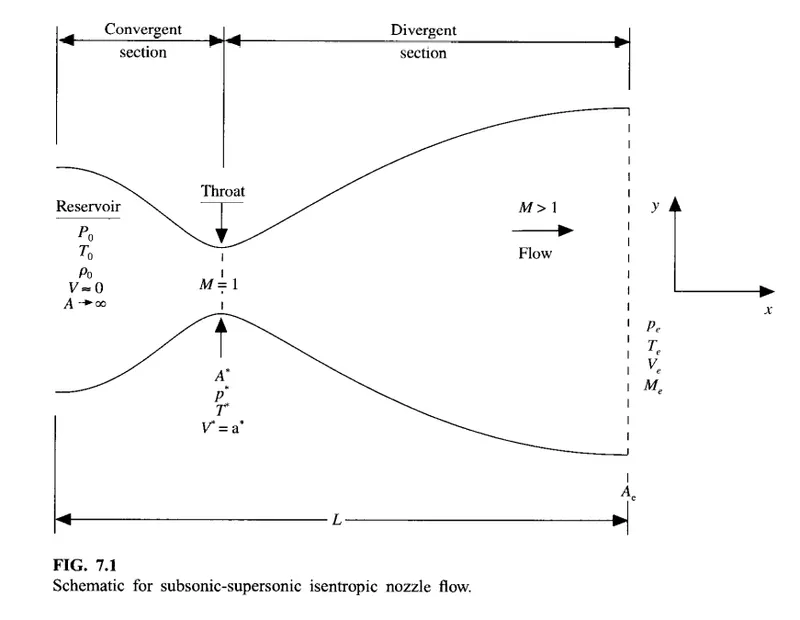
The diagramtic representation of the problem is given
EXPLANATION ;
NON CONSERVATIVE FORM -
- In non conservative form the primitive variables alone taken inside the partial operator ,secondary variables are taken out from partial . This is done as the non conservative form equation heads to dependence of the primitive variables of the function alone



CONSERVATIVE FORM
- In conservative form all the variables depends on the derivative function (i.e all the variables in the equation is dependent with partial operator and both primary and secondary variables are included inside the partial operator ) . This is done as the term is completely dependent to the derivative which corresponds to time or flex positions.
- Namley the conservative form of equations are identified variable vectors with solution vectors, flex vectors, source vectors
- continuity -`(delta(rhoA))/(deltat) +(delta(rhoAV))/(deltax) =0`
- momentum - `(delta(rhoAV))/(deltat) +(delta[(rhoAV^2)+(1/gamma)PA]/(deltax)) =(1/gamma)P((deltaA)/(deltax))`
- `(delta(rho((e)/(gamma -1)+((gamma)/(2)V^2)A)))/(deltat) + (delta(rho((e)/(gamma -1)+((gamma)/(2)V^2)VA+PAV)))/(deltat) = 0`
These governing equations are made dimensionless for the approach
CODE;
The code is given by calling two functions with recommended function inputs for it , These two function distincts for conservative and non conservative form.
MAIN CODE
function [Mass_flow_rate_C, Pressure_C, Mach_number_C,  rho_C, v_C, T_C, rho_throat_C, v_throat_C, T_throat_C, Mass_flow_rate_throat_C, Pressure_throat_C, Mach_number_throat_C] = Conservative_form(x, dx, n, gamma, nt, C)

%Determining Initial profile of Density and Temperature
for i = 1:n

    if (x(i) >= 0 && x(i) <= 0.5)
        rho_C(i) = 1;
        T_C(i) = 1;
    elseif (x(i) >= 0.5 && x(i) <= 1.5)
        rho_C(i) = 1 - 0.366*(x(i) - 0.5);
        T_C(i) = 1 - 0.167*(x(i) - 0.5);
    elseif (x(i) >= 1.5 && x(i) <= 3)
        rho_C(i) = 0.634 - 0.3879*(x(i) - 1.5);
        T_C(i) = 0.833 - 0.3507*(x(i) - 1.5);
    end

end

%Area & Throat profiles
a = 1 + 2.2*(x - 1.5).^2;
throat = find(a==1);

%Initial profile fot Velocity and Pressure
v_C = 0.59./(rho_C.*a);
Pressure_C = rho_C.*T_C;

%Calculate the Initial Solution Vectors(U)
U1 = rho_C.*a;
U2 = rho_C.*a.*v_C;
U3 = rho_C.*a.*(T_C./(gamma - 1)) + ((gamma/2).*v_C.^2);


%Outer Time Loop
for k =1:nt

    %Time-step control
    dt = min(C.*dx./(sqrt(T_C) + v_C));

    %Saving a copy of Old Values
    U1_old = U1;
    U2_old = U2;
    U3_old = U3;

    %Calculating the Flux vector(F)
    F1 = U2;
    F2 = ((U2.^2)./U1) + ((gamma - 1)/gamma)*(U3 - (gamma/2)*((U2.^2)./U1));
    F3 = ((gamma*U2.*U3)./U1) - (gamma*(gamma - 1)*((U2.^3)./(2*U1.^2)));


    %Predictor Method
    for j = 2:n-1

        %Calculating the Source term(J)
        J2(j) = (1/gamma)*rho_C(j)*T_C(j)*((a(j + 1) - a(j))/dx);


        %Continuity Equation
        dU1_dt_P(j) = -((F1(j + 1) - F1(j))/dx);

        %Momentum Equation
        dU2_dt_P(j) = -((F2(j + 1) - F2(j))/dx) + J2(j);

        %Energy Equation
        dU3_dt_P(j) = -((F3(j + 1) - F3(j))/dx);


        %Updating New values
        U1(j) = U1(j) + dU1_dt_P(j)*dt;
        U2(j) = U2(j) + dU2_dt_P(j)*dt;
        U3(j) = U3(j) + dU3_dt_P(j)*dt;

    end

    %Updating Flux vectors
    F1 = U2;
    F2 = ((U2.^2)./U1) + ((gamma - 1)/gamma)*(U3 - ((gamma*0.5*(U2.^2))./(U1)));
    F3 = ((gamma*U2.*U3)./U1) - ((gamma*0.5*(gamma - 1)*(U2.^3))./(U1.^2));


    %Corrector Method
    for j = 2:n-1

        %Updating the Source term(J)
        J2(j) = (1/gamma)*rho_C(j)*T_C(j)*((a(j) - a(j - 1))/dx);

        %Simplifying the Equation's spatial terms
        dU1_dt_C(j) = -((F1(j) - F1(j - 1))/dx);
        dU2_dt_C(j) = -((F2(j) - F2(j - 1))/dx) + J2(j);
        dU3_dt_C(j) = -((F3(j) - F3(j - 1))/dx);

    end

    %Compute Average Time derivative
    dU1_dt = 0.5*(dU1_dt_P + dU1_dt_C);
    dU2_dt = 0.5*(dU2_dt_P + dU2_dt_C);
    dU3_dt = 0.5*(dU3_dt_P + dU3_dt_C);

    %Final Solution Update
    for i = 2:n-1
        U1(i) = U1_old(i) + dU1_dt(i)*dt;
        U2(i) = U2_old(i) + dU2_dt(i)*dt;
        U3(i) = U3_old(i) + dU3_dt(i)*dt;

    end


    %Applying Boundary Conditions
    %At Inlet
    U1(1) = rho_C(1)*a(1);
    U2(1) = 2*U2(2) - U2(3);

    v_C(1) = U2(1)./U1(1);
    U3(1) = U1(1)*((T_C(1)/(gamma - 1)) + ((gamma/2)*(v_C(1)).^2));

    %At Outlet
    U1(n) = 2*U1(n - 1) - U1(n - 2);
    U2(n) = 2*U2(n - 1) - U2(n - 2);
    U3(n) = 2*U3(n - 1) - U3(n - 2);

    %Final Primitive value update
    rho_C = U1./a;
    v_C = U2./U1;
    T_C = (gamma - 1)*((U3./U1 - (gamma/2)*(v_C).^2));

    %Defining Mass flow rate, Pressure and Mach number
    Mass_flow_rate_C = rho_C.*a.*v_C;
    Pressure_C = rho_C.*T_C;
    Mach_number_C = (v_C./sqrt(T_C));

    %Calculating Variables at throat section
    rho_throat_C(k) = rho_C(throat);
    T_throat_C(k) = T_C(throat);
    v_throat_C(k) = v_C(throat);
    Mass_flow_rate_throat_C(k) = Mass_flow_rate_C(throat);
    Pressure_throat_C(k) = Pressure_C(throat);
    Mach_number_throat_C(k) = Mach_number_C(throat);

    %PLOTTING
    %Comparison of non-dimensional Mass flow rates at different time steps
    figure(2)
    if k == 50
       plot(x, Mass_flow_rate_C, 'y', 'linewidth', 1.25);
       hold on
    elseif k == 100
       plot(x, Mass_flow_rate_C, 'g', 'linewidth', 1.25);
       hold on
    elseif k == 200
       plot(x, Mass_flow_rate_C, 'c', 'linewidth', 1.25);
       hold on
    elseif k == 400
       plot(x, Mass_flow_rate_C, 'm', 'linewidth', 1.25);
       hold on
    elseif k == 800
       plot(x, Mass_flow_rate_C, 'k', 'linewidth', 1.25);
       hold on
    end


    %Labelling
    title('Mass flow rates at different Timesteps - CONSERVATIVE FORM')
    xlabel('Distance')
    ylabel('Mass flow rate')
    legend({'50^t^h Timestep','100^t^h Timestep','200^t^h Timestep','400^t^h Timestep','800^t^h Timestep'})
    axis([0 3 0.4 1])
    grid on

end

end
Function;
non conservative form
function [Mass_flow_rate_NC, Pressure_NC, Mach_number_NC, rho_NC, v_NC, T_NC, rho_throat_NC, v_throat_NC, T_throat_NC, Mass_flow_rate_throat_NC, Pressure_throat_NC, Mach_number_throat_NC] = Non_conservative_form(x, dx, n, gamma, nt, C)

%Intial boundary conditions
rho_NC = 1 - 0.3146*x;
T_NC = 1 - 0.2341*x;
v_NC = (0.1 + 1.09*x).*T_NC.^0.5;

%Area & Throat profiles
a = 1 + 2.2*(x - 1.5).^2;
throat = find(a==1);


%Outer Time Loop
for k = 1:nt

    %Time-step control
    dt = min(C.*dx./(sqrt(T_NC) + v_NC));

    %Saving a copy of Old Values
    rho_old = rho_NC;
    T_old = T_NC;
    v_old = v_NC;


    %Predictor Method
    for j = 2:n-1

        %Simplifying the Equation's spatial terms
        dv_dx = (v_NC(j + 1) - v_NC(j))/dx;
        drho_dx = (rho_NC(j + 1) - rho_NC(j))/dx;
        dT_dx = (T_NC(j + 1) - T_NC(j))/dx;
        dlog_a_dx = (log(a(j + 1)) - log(a(j)))/dx;

        %Continuity Equation
        drho_dt_P(j) = -rho_NC(j)*dv_dx - rho_NC(j)*v_NC(j)*dlog_a_dx - v_NC(j)*drho_dx;

        %Momentum Equation
        dv_dt_P(j) = -v_NC(j)*dv_dx - (1/gamma)*(dT_dx + (T_NC(j)*drho_dx/rho_NC(j)));

        %Energy Equation
        dT_dt_P(j) = -v_NC(j)*dT_dx - (gamma - 1)*T_NC(j)*(dv_dx + v_NC(j)*dlog_a_dx);


        %Solution Update
        rho_NC(j) = rho_NC(j) + drho_dt_P(j)*dt;
        v_NC(j) = v_NC(j) + dv_dt_P(j)*dt;
        T_NC(j) = T_NC(j) + dT_dt_P(j)*dt;

    end


    %Corrector Method
    for j = 2:n-1

        %Simplifying the Equation's spatial terms
        dv_dx = (v_NC(j) - v_NC(j - 1))/dx;
        drho_dx = (rho_NC(j) - rho_NC(j - 1))/dx;
        dT_dx = (T_NC(j) - T_NC(j - 1))/dx;
        dlog_a_dx = (log(a(j)) - log(a(j - 1)))/dx;

        %Continuity Equation
        drho_dt_C(j) = - rho_NC(j)*dv_dx - rho_NC(j)*v_NC(j)*dlog_a_dx - v_NC(j)*drho_dx;

        %Momentum Equation
        dv_dt_C(j) = - v_NC(j)*dv_dx - (1/gamma)*(dT_dx + (T_NC(j)*drho_dx/rho_NC(j)));

        %Energy Equation
        dT_dt_C(j) = - v_NC(j)*dT_dx - (gamma - 1)*T_NC(j)*(dv_dx + v_NC(j)*dlog_a_dx);

    end

    %Compute Average Time derivative
    drho_dt = 0.5.*(drho_dt_P + drho_dt_C);
    dv_dt = 0.5.*(dv_dt_P + dv_dt_C);
    dT_dt = 0.5.*(dT_dt_P + dT_dt_C);

    %Final Solution Update
    for i = 2:n-1
        rho_NC(i) = rho_old(i) + drho_dt(i)*dt;
        v_NC(i) = v_old(i) + dv_dt(i)*dt;
        T_NC(i) = T_old(i) + dT_dt(i)*dt;

    end

    %Applying Boundary Conditions
    %At Inlet
    rho_NC(1) = 1;
    v_NC(1) = 2*v_NC(2) - v_NC(3);
    T_NC(1) = 1;

    %At Outlet
    rho_NC(n) = 2*rho_NC(n-1) - rho_NC(n - 2);
    v_NC(n) = 2*v_NC(n - 1) - v_NC(n - 2);
    T_NC(n) = 2*T_NC(n - 1) - T_NC(n - 2);


    %Defining Mass flow rate, Pressure and Mach number
    Mass_flow_rate_NC = rho_NC.*a.*v_NC;
    Pressure_NC = rho_NC.*T_NC;
    Mach_number_NC = (v_NC./sqrt(T_NC));

    %Calculating Variables at throat section
    rho_throat_NC(k) = rho_NC(throat);
    T_throat_NC(k) = T_NC(throat);
    v_throat_NC(k) = v_NC(throat);
    Mass_flow_rate_throat_NC(k) = Mass_flow_rate_NC(throat);
    Pressure_throat_NC(k) = Pressure_NC(throat);
    Mach_number_throat_NC(k) = Mach_number_NC(throat);


    %PLOTTING
    %Comparison of non-dimensional Mass flow rates at different time steps
    figure(1);
    if k == 50
       plot(x, Mass_flow_rate_NC, 'y', 'linewidth', 1.25);
       hold on
    elseif k == 100
       plot(x, Mass_flow_rate_NC, 'g', 'linewidth', 1.25);
       hold on
    elseif k == 200
       plot(x, Mass_flow_rate_NC, 'c', 'linewidth', 1.25);
       hold on
    elseif k == 400
       plot(x, Mass_flow_rate_NC, 'm', 'linewidth', 1.25);
       hold on
    elseif k == 800
       plot(x, Mass_flow_rate_NC, 'k', 'linewidth', 1.25);
       hold on
    end

    %Labelling
    title('Mass flow rates at different Timesteps - NON CONSERVATIVE FORM)')
    xlabel('Distance')
    ylabel('Mass flow rate')
    legend({'50^t^h Timestep','100^t^h Timestep','200^t^h Timestep','400^t^h Timestep','800^t^h Timestep'})
    axis([0 3 0 2])
    grid on

end

end
conservative form
function [Mass_flow_rate_C, Pressure_C, Mach_number_C,  rho_C, v_C, T_C, rho_throat_C, v_throat_C, T_throat_C, Mass_flow_rate_throat_C, Pressure_throat_C, Mach_number_throat_C] = Conservative_form(x, dx, n, gamma, nt, C)

%Determining Initial profile of Density and Temperature
for i = 1:n

    if (x(i) >= 0 && x(i) <= 0.5)
        rho_C(i) = 1;
        T_C(i) = 1;
    elseif (x(i) >= 0.5 && x(i) <= 1.5)
        rho_C(i) = 1 - 0.366*(x(i) - 0.5);
        T_C(i) = 1 - 0.167*(x(i) - 0.5);
    elseif (x(i) >= 1.5 && x(i) <= 3)
        rho_C(i) = 0.634 - 0.3879*(x(i) - 1.5);
        T_C(i) = 0.833 - 0.3507*(x(i) - 1.5);
    end

end

%Area & Throat profiles
a = 1 + 2.2*(x - 1.5).^2;
throat = find(a==1);

%Initial profile fot Velocity and Pressure
v_C = 0.59./(rho_C.*a);
Pressure_C = rho_C.*T_C;

%Calculate the Initial Solution Vectors(U)
U1 = rho_C.*a;
U2 = rho_C.*a.*v_C;
U3 = rho_C.*a.*(T_C./(gamma - 1)) + ((gamma/2).*v_C.^2);


%Outer Time Loop
for k =1:nt

    %Time-step control
    dt = min(C.*dx./(sqrt(T_C) + v_C));

    %Saving a copy of Old Values
    U1_old = U1;
    U2_old = U2;
    U3_old = U3;

    %Calculating the Flux vector(F)
    F1 = U2;
    F2 = ((U2.^2)./U1) + ((gamma - 1)/gamma)*(U3 - (gamma/2)*((U2.^2)./U1));
    F3 = ((gamma*U2.*U3)./U1) - (gamma*(gamma - 1)*((U2.^3)./(2*U1.^2)));


    %Predictor Method
    for j = 2:n-1

        %Calculating the Source term(J)
        J2(j) = (1/gamma)*rho_C(j)*T_C(j)*((a(j + 1) - a(j))/dx);


        %Continuity Equation
        dU1_dt_P(j) = -((F1(j + 1) - F1(j))/dx);

        %Momentum Equation
        dU2_dt_P(j) = -((F2(j + 1) - F2(j))/dx) + J2(j);

        %Energy Equation
        dU3_dt_P(j) = -((F3(j + 1) - F3(j))/dx);


        %Updating New values
        U1(j) = U1(j) + dU1_dt_P(j)*dt;
        U2(j) = U2(j) + dU2_dt_P(j)*dt;
        U3(j) = U3(j) + dU3_dt_P(j)*dt;

    end

    %Updating Flux vectors
    F1 = U2;
    F2 = ((U2.^2)./U1) + ((gamma - 1)/gamma)*(U3 - ((gamma*0.5*(U2.^2))./(U1)));
    F3 = ((gamma*U2.*U3)./U1) - ((gamma*0.5*(gamma - 1)*(U2.^3))./(U1.^2));


    %Corrector Method
    for j = 2:n-1

        %Updating the Source term(J)
        J2(j) = (1/gamma)*rho_C(j)*T_C(j)*((a(j) - a(j - 1))/dx);

        %Simplifying the Equation's spatial terms
        dU1_dt_C(j) = -((F1(j) - F1(j - 1))/dx);
        dU2_dt_C(j) = -((F2(j) - F2(j - 1))/dx) + J2(j);
        dU3_dt_C(j) = -((F3(j) - F3(j - 1))/dx);

    end

    %Compute Average Time derivative
    dU1_dt = 0.5*(dU1_dt_P + dU1_dt_C);
    dU2_dt = 0.5*(dU2_dt_P + dU2_dt_C);
    dU3_dt = 0.5*(dU3_dt_P + dU3_dt_C);

    %Final Solution Update
    for i = 2:n-1
        U1(i) = U1_old(i) + dU1_dt(i)*dt;
        U2(i) = U2_old(i) + dU2_dt(i)*dt;
        U3(i) = U3_old(i) + dU3_dt(i)*dt;

    end


    %Applying Boundary Conditions
    %At Inlet
    U1(1) = rho_C(1)*a(1);
    U2(1) = 2*U2(2) - U2(3);

    v_C(1) = U2(1)./U1(1);
    U3(1) = U1(1)*((T_C(1)/(gamma - 1)) + ((gamma/2)*(v_C(1)).^2));

    %At Outlet
    U1(n) = 2*U1(n - 1) - U1(n - 2);
    U2(n) = 2*U2(n - 1) - U2(n - 2);
    U3(n) = 2*U3(n - 1) - U3(n - 2);

    %Final Primitive value update
    rho_C = U1./a;
    v_C = U2./U1;
    T_C = (gamma - 1)*((U3./U1 - (gamma/2)*(v_C).^2));

    %Defining Mass flow rate, Pressure and Mach number
    Mass_flow_rate_C = rho_C.*a.*v_C;
    Pressure_C = rho_C.*T_C;
    Mach_number_C = (v_C./sqrt(T_C));

    %Calculating Variables at throat section
    rho_throat_C(k) = rho_C(throat);
    T_throat_C(k) = T_C(throat);
    v_throat_C(k) = v_C(throat);
    Mass_flow_rate_throat_C(k) = Mass_flow_rate_C(throat);
    Pressure_throat_C(k) = Pressure_C(throat);
    Mach_number_throat_C(k) = Mach_number_C(throat);

    %PLOTTING
    %Comparison of non-dimensional Mass flow rates at different time steps
    figure(2)
    if k == 50
       plot(x, Mass_flow_rate_C, 'y', 'linewidth', 1.25);
       hold on
    elseif k == 100
       plot(x, Mass_flow_rate_C, 'g', 'linewidth', 1.25);
       hold on
    elseif k == 200
       plot(x, Mass_flow_rate_C, 'c', 'linewidth', 1.25);
       hold on
    elseif k == 400
       plot(x, Mass_flow_rate_C, 'm', 'linewidth', 1.25);
       hold on
    elseif k == 800
       plot(x, Mass_flow_rate_C, 'k', 'linewidth', 1.25);
       hold on
    end


    %Labelling
    title('Mass flow rates at different Timesteps - CONSERVATIVE FORM')
    xlabel('Distance')
    ylabel('Mass flow rate')
    legend({'50^t^h Timestep','100^t^h Timestep','200^t^h Timestep','400^t^h Timestep','800^t^h Timestep'})
    axis([0 3 0.4 1])
    grid on

end

end
CODE EXPLANATION ;
- Two functions for conservative and nonservative method is made to simulate individually and to compare the study with a graph
- Function defintion is made with the terms corresponds to time step variations and the nodal position of the nozzle , then the primitive variable terms are defined inside the definition
- Solution of the code corresponds with meshing , discritzing and solving the governing equation by macormakl method
- The governing terms are made dimensioless to solve the system
- Initial conditions of the variables are specified with the equations depending on the x position of the nozzle and they are set relocate as the old referred values (i.e Nth step variable when the sysytem approaches N+1TH STEP)
- Time loop for the system is given and the internal nodes where the equation approaches for the next time derivative is given by allocating the number of nodes to 31
- Area is dependent of x in this system considerably so every equation having variables dependent on x
Predictor method :
Here the term approaching for the next time step is forward differnced with space terms and the output from this leads to predictor time derivative . This term is upadated with the initial term and this updated term procceeds for corrector step
Corrector step :
Here the spatial term goes through backward differncing of the equation and corresponds to `Deltat`time step
Averaging :
Here both the time steps are averaged combinedly and thei avg value is added with the previous reffered time step vale of the variables . THis time step follows for the Nth time step mentioned
In conservative from variables comes under partial derivations as the variables here are substituted to identify as solution vectors, source vectors and flec vectors for performing the macormak method of solving
- Boundary conditions are mentioned as the system needs flow field conditions at inflow and at outflow boundaries
- primitive variables are found with the relative equations from the variables
- a graph plotting the mass flow rate at certain time step is compared in a single figure
PLOTS;
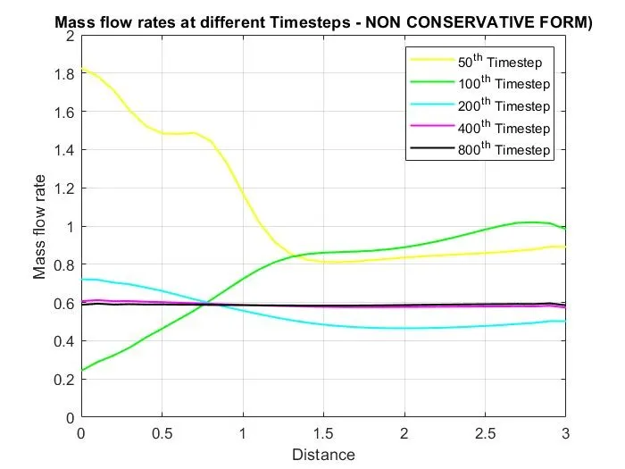
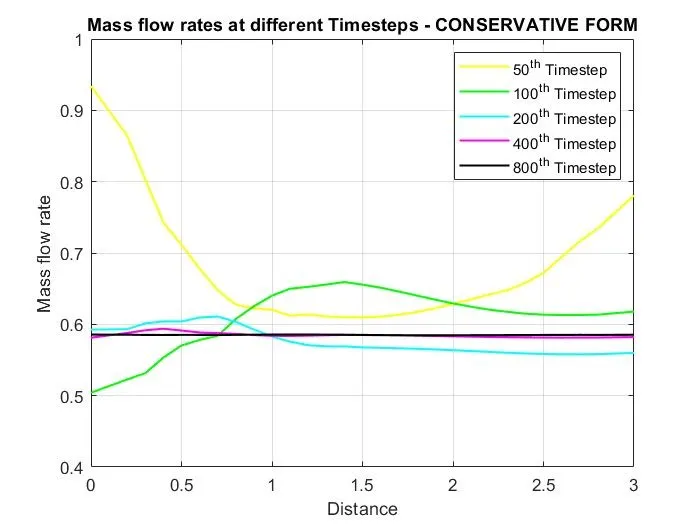
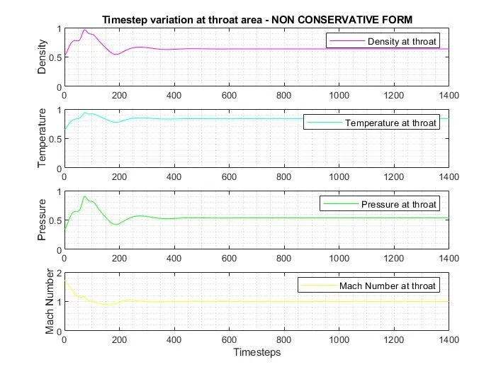
OBSERVATION :
- Taking Time step variation in consideration for both the flow - Conservative form reaches a stabilised flow variables at shorter time steps when compared to non conservative form
- Taking flow rate distribution in account both the forms perform similar to the solution discritized respectively
- Mass flow rate curve comparison gives a enormous variation in graph as conservative form is more stablised and calm performing within boundary condition when compared with non conservative term
- As the time step approches to the end the flow rates gets into steady shape and continues to flow stable after 400th time step.
GRID
INFERENCE:
Grid test is taken for internal nodal meshin when n=31 and n=61 and the flow distribution variables are taken and compared within the box. This test is taken as the problem solved can be checked for time rates and checked for stability as here the variables are plotting similar values even when the meshing gets the double sized for the simulation . This test is grid dependant
Considering conservative and non conservative form os solving Conserving time steps are more quicker and stable .