Week 4.1 - Genetic Algorithm

OBJECTIVE

To understand the concept of genetic algorithm and execute a program finding the optimised global maxima of the stalagmite function

GENETIC ALGORITHM

• genetic algorithm is derived from Charle Darwin's Evolutionary theory
• The algorithm randomly selects the individuals for the optimisation from the population
• Repeatedly modifies the population of the individual solution
• Used for optimising the function for finding maxima and minima

WORKING

• CREATE INITIAL RANDOM POPULATION OF ORGANISMS
• IT CHECKS IF THE OPTIMAL SOLUTION OR THE DESERVED SOLUTION HAD COME OUT OR NOT

IF YES - END

IF NO

• REPRODUCE THE ORGANISMS
• THEN MUTATE THEM TO FOLLOW THE SAME PROCESS OF FINDING THE OPTIMAL SOLUTION

GA command finds the optimal individual organisms by following three process

• SELECTION OPERATOR
• CROSSOVER OPERATOR
• MUTATION OPERATOR

OPTIMISATION

• Optimisation is the process of deriving the best , suitable solution depending to various multi parameters of the solution
• Through optimisation we can find the deserved maximum and minimum of the function

MATLAB PROGRAM TO FIND THE GLOBAL MAXIMUM OF THE FUNCTION USING GA

THE PROGRAM to find the surface plot of x,y,f behaving to the GA for the function stalagmite

close all %closes the previous tabs,figs
clear all %clears the workspace variable info
clc %clears the command window

% mesh grid
x = linspace(0,0.6,150)
y = linspace(0,0.6,150)

[xx,yy] = meshgrid(x,y);

for i = 1:length(xx)
    for j =1:length(yy)
        input_vector(1) = xx(i,j);
        input_vector(2) = yy(i,j);
        f(i,j) = stalagmite(input_vector);
    end
end


surf(xx,yy,f);
shading interp
xlabel('x axis');
ylabel('y axis');
title('plot of x,y,f');


[inputs,fval] = ga(@stalagmite,2)

THE FUNCTION

% function stalagmite
function [f] = stalagmite(input_vector)

x = input_vector(1);
y = input_vector(2);

f1x = (sin((5.1*pi*x) + 0.5))^6;
f1y = (sin((5.1*pi*y) + 0.5))^6;
f2x = exp(-4*log(2)*((x-0.0667)^2)/0.64);
f2y = exp(-4*log(2)*((y-0.0667)^2)/0.64);

f = -(f1x*f2x*f1y*f2y);

EXPLANATION

THE FUNCTION STALAGMITE

From the mathematical formula given for finding the (x,y) of function stalagmite , The paramters F(X1) F(X2) F(Y1) F(Y2) have been assigned and substituted inside the function stalagmite.

EXPLANATION

PROGRAM

initial values of x and y have been set to have 150 values and formed a 2d array by giving a command 'meshgrid'

This command helps to form the 2d arrays of x and y in [xx yy]

• For (x,y) places in the 2d array the stalagmite function is called corresponding to all the points of (x,y)
• Then plot command is followed to view the function in a surface form by giving surf command
• This reults in a formation stalagmites having the values of (x,y) which undergoes the function stalagmite . so the 3D image has (x,y,z0 values at all points in the surface

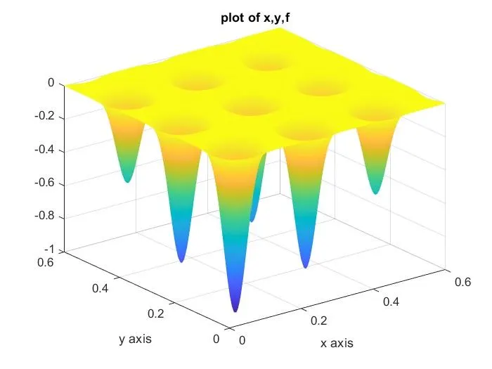
• GA determines the minimum value by default for the x and y inputs of the function
• here fval = -0.573
• inputs x = -0.132
• inputs y = 0.045

CASE 1

MATLAB PROGRAM OF GA WITHOUT BOUNDED RANGE

THE PROGRAM

close all %closes the previous tabs,figs
clear all %clears the workspace variable info
clc %clears the command window

% mesh grid
x = linspace(0,0.6,150)
y = linspace(0,0.6,150)

[xx,yy] = meshgrid(x,y);

for i = 1:length(xx)
    for j =1:length(yy)
        input_vector(1) = xx(i,j);
        input_vector(2) = yy(i,j);
        f(i,j) = stalagmite(input_vector);
    end
end


% no of iterations
num_cases = 50

% study time
tic

% study case 1 (with iterations, unbounded input range)
for i = 1:num_cases;
[inputs,fopt(i)]= ga(@stalagmite,2);
xopt(i)=inputs(1);
yopt(i)=inputs(2);
end


study1_time =toc %used for estimating the time in seconds for the program

figure (1)
subplot(2,1,1) % 2 ROWS, 1 COLUMN , 1 POSITION
hold on 
surf(xx,yy,f)
shading interp %AVOIDS THE LINE INTERFACE
hold on 
plot3(xopt,yopt,fopt,'marker','o','markersize',3,'MarkerFaceColor','r')
title('unbounded input range') %TITLE NAME
subplot(2,1,2) % 2 ROWS , 2 COLUMN , 2 POSITION
hold on 
plot(fopt) % PLOTS F OPTIMISED DATA IN  GRAPH WITH REFERENCE TO ITERATIONS
xlabel('iterations')
ylabel('function minimum')

EXPLANATION

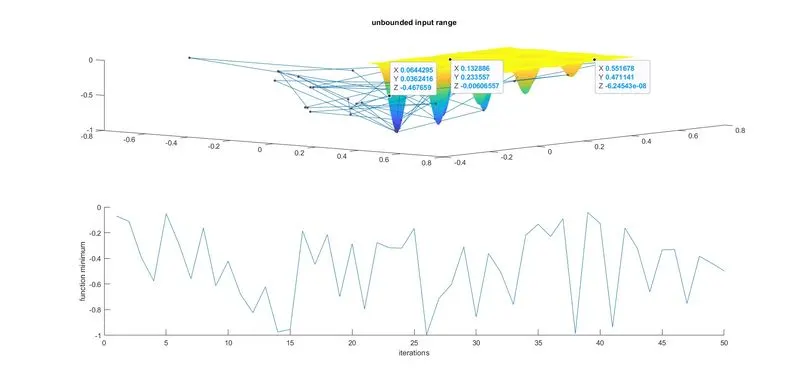
• IN this program we have set the program to repeat 50 times to see the behaviour of the function every 50 times so that the GA results in different maxima values by selecting the random indiviuals and proceeding for the cross over for each 50 times
• So that we get different values of maxima and inputs and the positioning of the minima values could be seen in the 3d figure below
• to repeat the program for 50 times and note the time limit 'tic - for loop (for which the time has to be taken ) -toc' is used
• the program has xopt,yopt,fopt values in 3d surface with lines denoting the values of fval for 50 times, 'PLOT3 is used to give the image in 3d 3 axis
• fopt for 50 iterations , this data has been separately plotted to understand the change of fopt for 50 iterations

THE FIGURE

CASE 2

MATLAB PROGRAM OF GA WITH BOUNDED RANGE

• In this program weh run thr GA matlab program for finding the global maxima with bounded range of inputs
• first we gave to take the reference population from the x and y limits having 150 values of independent population size and range.
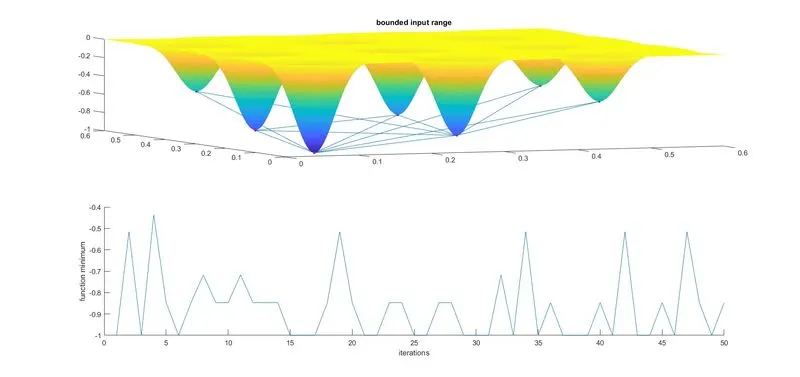
• Here we tell the GA to take the population from certain range of limits corresponding to x and y values so that the GA proceeds in a much controlled way of approaching the optimisation of the program
• we use num_cases for iterations
• and time taken is derived from 'tic' and 'toc' comments
• the program has xopt,yopt,fopt values in 3d surface with lines denoting the values of fval for 50 times
• fopt for 50 iterations , this data has been separately plotted to understand the change of fopt for 50 iterations

THE PROGRAM

close all %closes the previous tabs,figs
clear all %clears the workspace variable info
clc %clears the command window


% mesh grid
x = linspace(0,0.6,150)
y = linspace(0,0.6,150)

[xx,yy] = meshgrid(x,y);

for i = 1:length(xx)
    for j =1:length(yy)
        input_vector(1) = xx(i,j);
        input_vector(2) = yy(i,j);
        f(i,j) = stalagmite(input_vector);
    end
end


% no of iterations
num_cases = 50

% study time
tic

% study case 2 (with iterations, bounded input range)
for i = 1:num_cases;
[inputs,fopt(i)]= ga(@stalagmite,2,[],[],[],[],[0;0],[2;2]);
xopt(i)=inputs(1);
yopt(i)=inputs(2);
end

study2_time =toc %used for estimating the time in seconds for the program



[inputs,fval] = ga(@stalagmite,2)

% study case 2 (with iterations, unbounded input range)



figure (1)
subplot(2,1,1) % 2 ROWS, 1 COLUMN , 1 POSITION
hold on 
surf(xx,yy,f)
shading interp  %AVOIDS THE LINE INTERFACE
hold on 
plot3(xopt,yopt,fopt,'marker','o','markersize',3,'MarkerFaceColor','r')
title('bounded input range')
subplot(2,1,2) % 2 ROWS , 1 COLUMN , 2 POSITION
hold on 
plot(fopt) % PLOTS F OPTIMISED DATA IN  GRAPH WITH REFERENCE TO ITERATIONS
xlabel('iterations')
ylabel('function minimum')

the study time is 3.186 seconds

• THE syntax while calling the stalagmite for GA is discussed below

THE FIGURE

CASE 3

MATLAB PROGRAM OF GA TO FIND THE MAXIMA WITH BOOUNDED RANGE AND POPULATION SIZE

• In this case we set the GA to find the maxima results within a range and setting a populatiion size for the range
• By default the GA takes only 50 population for random sampling and crossover which leads to apoor end result
• By giving a range and specifying a population size , the GA determines to optimise the function in a narrow way to get more satisfying results
• This program tends to have a option syntax while calling the stalagmite function to specify the population size
• (input,fval)= ga(func,nvars,A,b,Aeq,beq,lb,ub,nonlcon,options)

(input,fval) - output of the stalagmite defining the inputs(x,y) and function values corresponding to x and y

Ga - calling the function (inbuild function)

func- function handle

nvars - number of variables

A - linear inequal constraints in matrix form of m rows and n columns ; m- no of equations (inequal form), n - number of variables
B - inear inequal constraints in vector form of m rows and n columns ; m- no of equations (inequal form),n - number of variables

Aeq - linear equal constraints in matrix form of m rows and n columns ; m- no of equations (inequal form), n - number of variables
Beq - inear equal constraints in vector form of m rows and n columns ; m- no of equations (inequal form),n - number of variables

lb- lower bound range for x and y

Ub- upper bound range for x and y

nonlcon - non linear constraints as a function name

options - options used to modify or add parameters like getting plots , adding population sizes for the GA reference

• this options syntax is first specified to follow with GA and then defining a paramater like population size
• this options is created by calling optimoptions

IF the program does not have any refernce for the syntax then the syntax is kept [] (blank) followed by other next syntax

THE PROGRAM

close all %closes the previous tabs,figs
clear all %clears the workspace variable info
clc %clears the command window 

% mesh grid
x = linspace(0,0.6,150)
y = linspace(0,0.6,150)

[xx,yy] = meshgrid(x,y);

for i = 1:length(xx)
    for j =1:length(yy)
        input_vector(1) = xx(i,j);
        input_vector(2) = yy(i,j);
        f(i,j) = stalagmite(input_vector);
    end
end
% no of iterations
num_cases = 50

% study time
tic
% population size inclusion by options command 
options = optimoptions('ga')
options = optimoptions(options,'PopulationSize',170);

% study case 3 (with iterations, bounded input range,population size)
for i = 1:num_cases;
[inputs,fopt(i)]= ga(@stalagmite,2,[],[],[],[],[0;0],[0.2;0.2],[],[],options);
xopt(i)=inputs(1);
yopt(i)=inputs(2);
end

study3_time =toc %used for estimating the time in seconds for the program
 

% study case 1 (with iterations, unbounded input range)



figure (1)
subplot(2,1,1) % 2 ROWS, 1 COLUMN , 1 POSITION
hold on 
surf(xx,yy,f)
shading interp  %AVOIDS THE LINE INTERFACE
hold on 
plot3(xopt,yopt,fopt,'marker','o','markersize',3,'MarkerFaceColor','r')
title('unbounded input range with population size')
subplot(2,1,2) % 2 ROWS , 1 COLUMN , 2 POSITION
hold on 
plot(fopt) % PLOTS F OPTIMISED DATA IN  GRAPH WITH REFERENCE TO ITERATIONS
xlabel('iterations')
ylabel('function minimum')

THE FIGURE

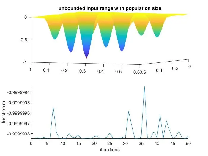
as it is clearly visible that the red marker constrains to the optimised global maxima(optima) of the stalagmites shown in the surface plots

PROBLEMS FACED while doing the challenge

I was not getting the the problem approach towards maximising . I GOT the stalagmites approach in a upside down way but the result took over the problem in a same opposite way .