Week 7 - Simulation of a 1D Supersonic nozzle flow simulation using Macormack Method
OBJECTIVE
To simulate and discuss the results of the isentropic flow in a nozzle with 1D supersonic flow, with help of solving the both conservative and non conservative forms of governing equation with help of Macormack Method using MATLAB.
RESULTS EXPECTED FOR:-
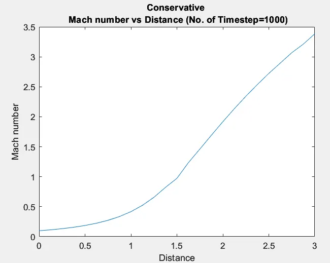
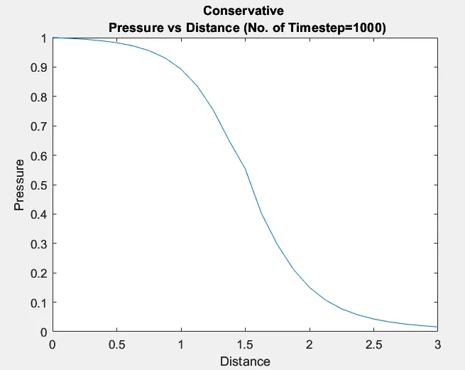
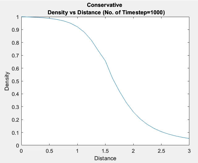
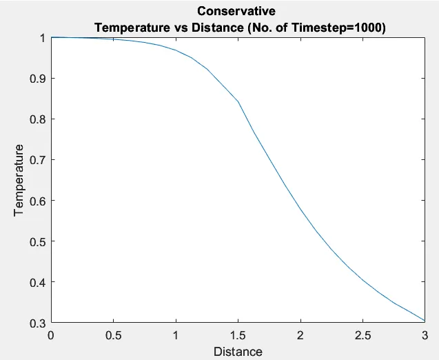
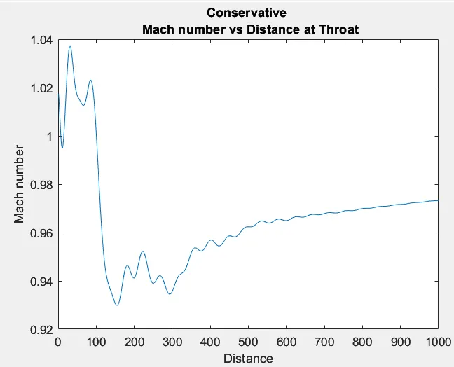
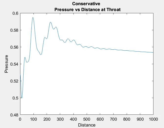
1) Steady State distribution of various flow parameters like Mach number, Pressure and Temperature.
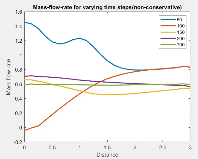
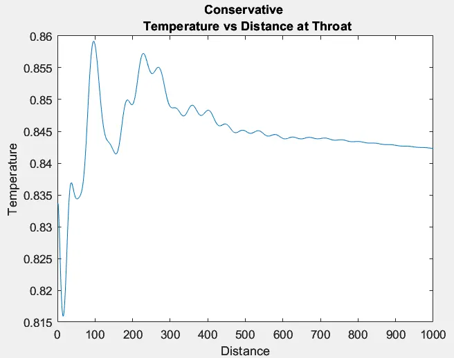
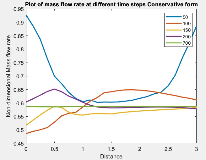
2) Time-Dependancy of various flow parameters like Mass Flow Rate.
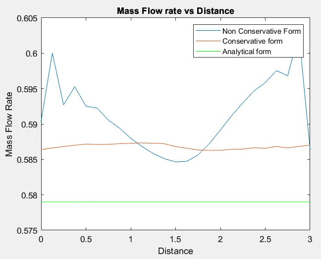
3) Comparison of results of conservative and non conservative forms.
THEORY
Nozzle:- It is a device used and designed to control the characteristics like pressure and velocity of flowing fluid. Generally the exit velocity is higher than the entering velocity of fluid which is achoeved with help of varying area (converging) inside the pipe/nozzle.
The Convergent Divergent nozzle is used in our case which results in the supersonic stream from low speed inlet. Mach number, the ratio of the speed of a body to the speed of sound in the surrounding medium, increases from 0 at inlet to Ma>1 at outlet.
The inlet is considered as a resevoir of fluid with stagnation values as-
Po = Inlet Pressure
To = Inlet Temperature
Ao = Inlet area (∞)
Vo = Inlet velocity (0)
Outlet conditions-
Pe = Outlet Pressure
Te = Outlet Temperature
Ve = Outlet velocity (0)
M = Mach number
At the converging region the throat we have subsonic flow (M=1) which means that the local velocity at this location is equal to the local speed of sound.
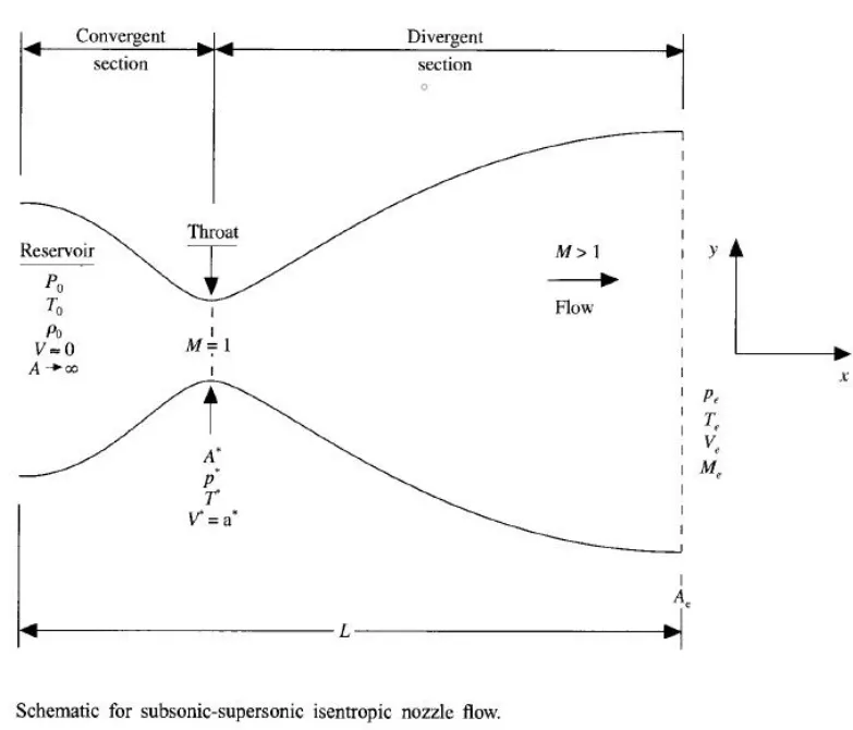
We will be assuming to have Quasi-1D-Flow which means that the properties won't change over the cross-section and remain uniform over all the cross section. Thus the flow properties will only change over the x distance (Unlike in reality).
SETUP/METHOD TO SOLVE
3 fundamental steps:-
Step 1) Mesh- Create 1D grid along x-axis.
Step 2) Discretize- Use Macormack method with help of time-marching method with predictor and corrector steps with help of initial conditions.
Step 3) Solve- Calculation of details at different time steps.
Mach number :
It is a dimensionless quantity representing the ratio of flow velocity to the local speed of the sound.
M=uc">M= u/c
M - Mach number.
u - Flow velocity.
c - Velocity of sound.
- At convergent section the flow velocity is less than the sound velocity therefore there mach number is less than 1.
- At throat section the flow velocity is equal to the sound velocity therefore there mach number is equal to 1.
- At divergent section the flow velocity is greater than the sound velocity therefore there mach number is greater than 1.
We will be solving the governing equations in 2 different forms:-
1) Non-Conservative
In this form the variables differentiated are coefficients of derivatives in an equation.



2) Consevative
In this form the variables differentiated are not the coefficients of any derivative in the equation.



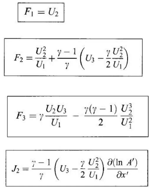
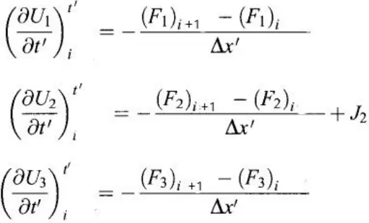
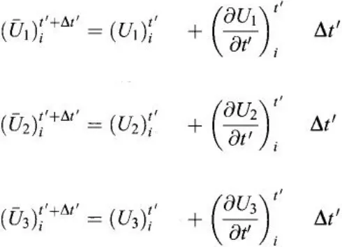
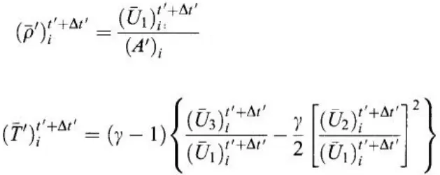
The all 3 above equations are non-dimentional generic equations for 1D Quasi Dimention Flow.
MacCormack method :
It is a second order accurate explicit finite difference technique for both space and time terms. It is a 3 step method to calculate a final numerical solution for an iteration involving following steps:-
1) Predictor Step- Forward differencing is done for spacial derivatives
2) Corrector Step- Backward differencing is done for spacial derivatives
3) Averaging Step- The solutions obtained from these 2 steps is averaged to give a single iteration.
FOR NON-CONSERVATIVE FORM
PREDICTOR STEP
We will do the forward differencing of spatial derivatives of generalized equtions:-



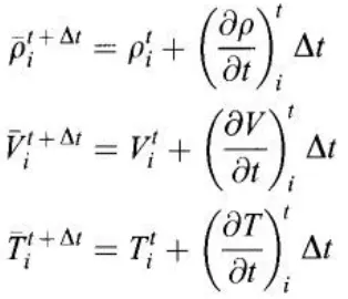
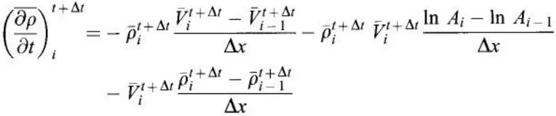

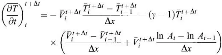
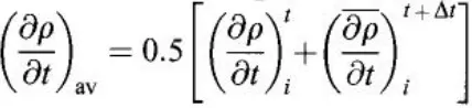
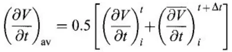
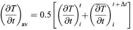
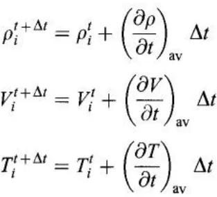
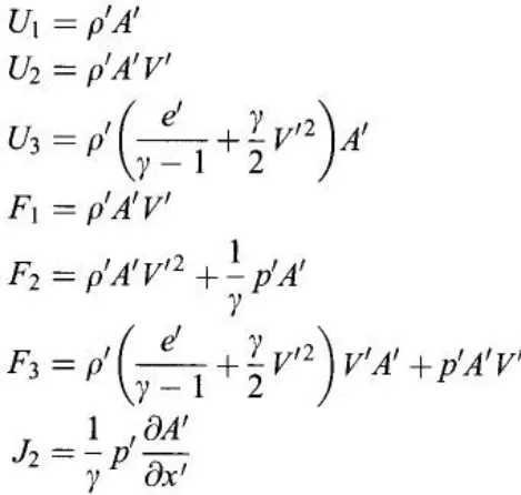
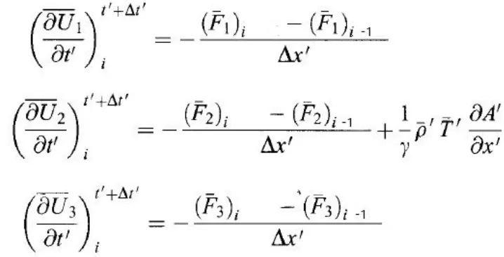
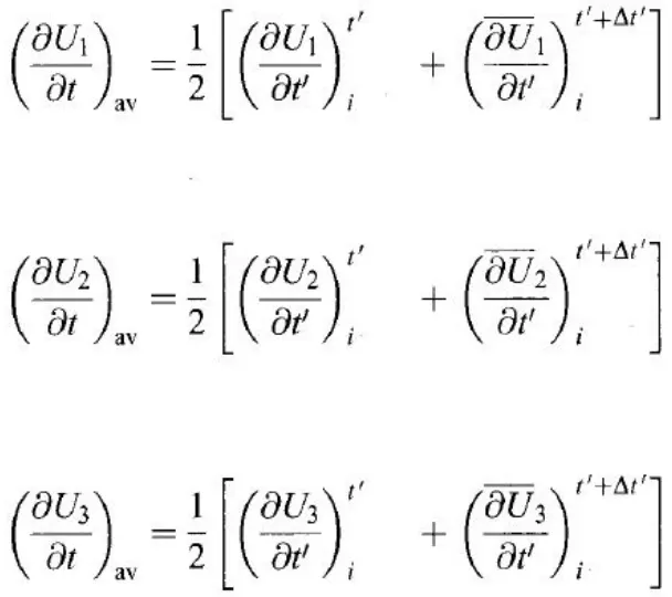
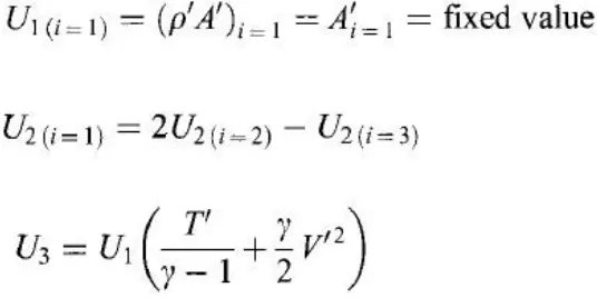
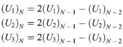
clear all
close all
clc

% Defining the time variables
n = 25; % grid points
nt = 1000; % num of time steps

% For non-conservative case
[rho,v,t,P,M,rho_t,v_t,t_t,P_t,M_t,x,a]=non_conservative(n,nt);

% for Conservative case
[rho_c,v_c,t_c,P_c,M_c,rho_t_c,v_t_c,t_t_c,P_t_c,M_t_c,x,a]=conservative(n,nt)

% Plotting

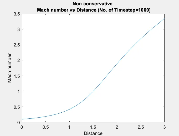
% Plots for Non Conservative, Mach number Vs distance at 1400 time step
figure()
plot(x,M)
title_text=sprintf('Non conservative \n Mach number vs Distance (No. of Timestep=%d)',nt);
title(title_text)
xlabel('Distance')
ylabel('Mach number')

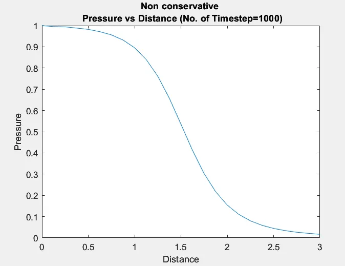
% Plots for Non Conservative,pressure Vs distance at 1400 time step
figure()
plot(x,P)
title_text=sprintf('Non conservative \n Pressure vs Distance (No. of Timestep=%d)',nt);
title(title_text)
xlabel('Distance')
ylabel('Pressure')

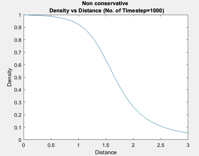
% Plots for Non Conservative, density Vs distance at 1400 time step
figure()
plot(x,rho)
title_text=sprintf('Non conservative \n Density vs Distance (No. of Timestep=%d)',nt);
title(title_text)
xlabel('Distance')
ylabel('Density')

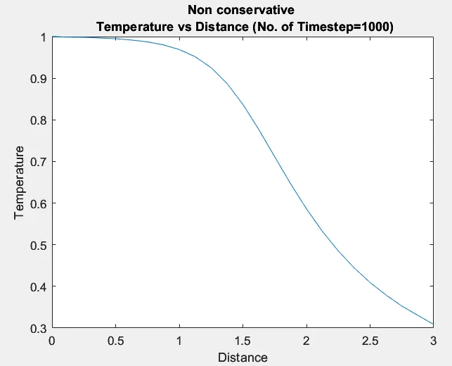
% Plots for Non Conservative, temperature Vs distance at 1400 time step
figure()
plot(x,t)
title_text=sprintf('Non conservative \n Temperature vs Distance (No. of Timestep=%d)',nt);
title(title_text)
xlabel('Distance')
ylabel('Temperature')

% Plots for Conservative, Mach number
figure()
plot(x,M_c)
title_text=sprintf('Conservative \n Mach number vs Distance (No. of Timestep=%d)',nt);
title(title_text)
xlabel('Distance')
ylabel('Mach number')

% Plots for Conservative,pressure Vs distance at 1400 time step
figure()
plot(x,P_c)
title_text=sprintf('Conservative \n Pressure vs Distance (No. of Timestep=%d)',nt);
title(title_text)
xlabel('Distance')
ylabel('Pressure')

% Plots for Conservative, density Vs distance at 1400 time step
figure()
plot(x,rho_c)
title_text=sprintf('Conservative \n Density vs Distance (No. of Timestep=%d)',nt);
title(title_text)
xlabel('Distance')
ylabel('Density')

% Plots for Conservative, temperature Vs distance at 1400 time step
figure()
plot(x,t_c)
title_text=sprintf('Conservative \n Temperature vs Distance (No. of Timestep=%d)',nt);
title(title_text)
xlabel('Distance')
ylabel('Temperature')

% Plots for Non Conservative
nt=(1:1000);

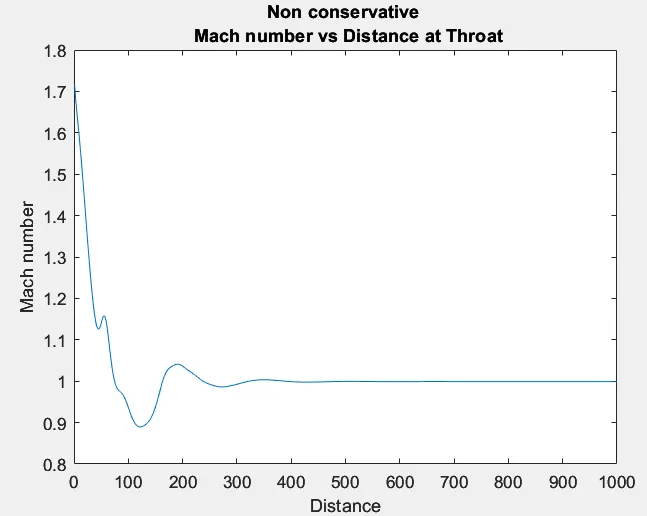
% Plots for Non Conservative, Mach number Vs distance at Throat area
figure()
plot(nt,M_t)
title_text=sprintf('Non conservative \n Mach number vs Distance at Throat');
title(title_text)
xlabel('Distance')
ylabel('Mach number')

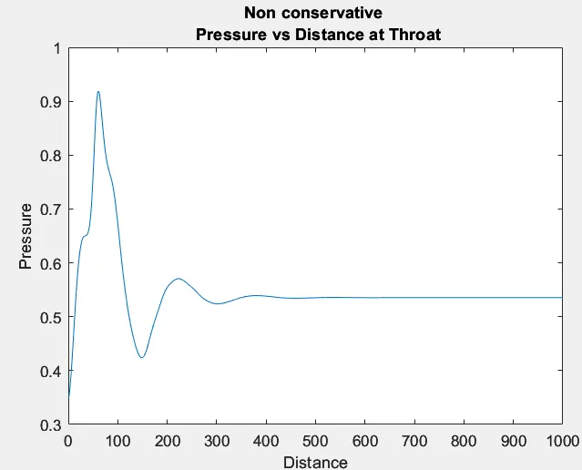
% Plots for Non Conservative, pressure Vs distance at Throat area
figure()
plot(nt,P_t);
title_text=sprintf('Non conservative \n Pressure vs Distance at Throat');
title(title_text)
xlabel('Distance')
ylabel('Pressure')
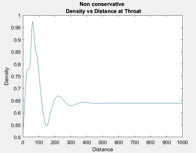
figure()
plot(nt,rho_t)
title_text=sprintf('Non conservative \n Density vs Distance at Throat');
title(title_text)
xlabel('Distance')
ylabel('Density')

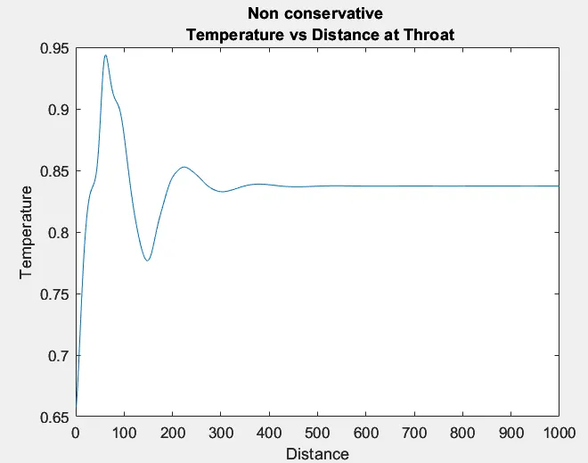
% Plots for Non Conservative, temperature Vs distance at Throat area
figure()
plot(nt,t_t)
title_text=sprintf('Non conservative \n Temperature vs Distance at Throat');
title(title_text)
xlabel('Distance')
ylabel('Temperature')

% Plots for Conservative

% Plots for Conservative, Mach number Vs distance at Throat area
figure()
plot(nt,M_t_c)
title_text=sprintf('Conservative \n Mach number vs Distance at Throat');
title(title_text)
xlabel('Distance')
ylabel('Mach number')

% Plots for Conservative, Pressure Vs distance at Throat area
figure()
plot(nt,P_t_c);
title_text=sprintf('Conservative \n Pressure vs Distance at Throat');
title(title_text)
xlabel('Distance')
ylabel('Pressure')
figure()
plot(nt,rho_t_c)
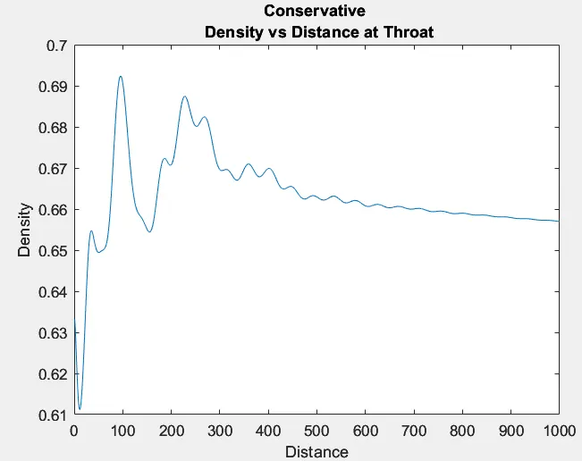
title_text=sprintf('Conservative \n Density vs Distance at Throat');
title(title_text)
xlabel('Distance')
ylabel('Density')

% Plots for Conservative, Mach Temperature Vs distance at Throat area
figure()
plot(nt,t_t_c)
title_text=sprintf('Conservative \n Temperature vs Distance at Throat');
title(title_text)
xlabel('Distance')
ylabel('Temperature')

% Ploting for mass flow rate distribution
figure()
m=rho.*a.*v;
m_c=rho_c.*a.*v_c;
plot(x,m)
hold on
plot(x,m_c)
line([0 3],[0.579 0.579],'color','g')
title_text=sprintf('Mass Flow rate vs Distance');
title(title_text)
% axis([0 3 .578 .596])
xlabel('Distance')
ylabel('Mass Flow Rate')
legend('Non Conservative Form','Conservative form','Analytical form')function [rho_c,v_c,t_c,P_c,M_c,rho_t_c,v_t_c,t_t_c,P_t_c,M_t_c,x,a]=conservative(n,nt)
%defining the inputs required
n=25;
x= linspace(0,3,n);
dx=x(2)-x(1);
%Calculating initial parameters
for i=1:length(x)
if (x(i)<=3.5)
t=0.833-0.3507*(x-1.5); % temperature
rho= 0.634-0.3879*(x-1.5); % density
end
end
% finding the parameters for different x distance values
for i=1:length(x)
if (x(i)<=1.5)
rho(i)=1.0-0.366*(x(i)-0.5) % density
t(i)=1.0-0.167*(x(i)-0.5) % Temperature
end
end
for i=1:length(x)
if (x(i)<=0.5)
rho(i)=1.0 % density
t(i)=1.0 % Temperature
end
end
% creating the velocity and area function to describe the nozzle
a=1+(2.2*(x-1.5).^2); % area
v=(.59)./(rho.*a); % velocity
gamma=1.4;
% no. of timestep
nt=1000;
% time step
delta_t=0.5*(dx./((sqrt(t)+v)));
dt=min(delta_t);
% defining the Solution Vector
U1=rho.*a;
U2=rho.*a.*v;
U3=rho.*((t./(gamma-1))+(gamma/2).*v.^2).*a;
% Defining the vectors for each time steps
for k=1:nt
U1_old=U1;
U2_old=U2;
U3_old=U3;
% Defining the Flux Vectors
F1=U2;
F2=((U2.^2)./U1)+((gamma-1)/gamma)*(U3-(gamma/2)*(((U2).^2)./U1));
F3=(((gamma)*(U2.*U3))./U1)-(((gamma*(gamma-1))/2)*((U2.^3)./U1.^2));
% creating loop for Predictor Steps
for j=2:n-1
J2(j)=(1/gamma)*rho(j)*t(j)*((a(j+1)-a(j))/dx);
dU1dt_p(j)=-((F1(j+1)-F1(j))/dx);
dU2dt_p(j)=-((F2(j+1)-F2(j))/dx)+J2(j);
dU3dt_p(j)=-((F3(j+1)-F3(j))/dx);
U1(j)=U1_old(j)+(dU1dt_p(j))*dt;
U2(j)=U2_old(j)+(dU2dt_p(j))*dt;
U3(j)=U3_old(j)+(dU3dt_p(j))*dt;
end
%uploading the solution
rho=(U1./a);
v=(U2./U1);
t= (gamma-1)*((U3./U1)-(gamma/2)*(v).^2);
%Updating the values of fluxes
%Flux Vector
F1=U2;
F2=((U2.^2)./U1)+((gamma-1)/gamma)*(U3-(gamma/2)*(((U2).^2)./U1));
F3=(((gamma)*(U2.*U3))./U1)-(((gamma*(gamma-1))/2)*((U2.^3)./U1.^2));
%loop for Corrector Step
for m=2:n-1
J2(m)=(1/gamma)*rho(m)*t(m)*((a(m)-a(m-1))/dx);
dU1dt_c(m)=-((F1(m)-F1(m-1))/dx);
dU2dt_c(m)=-((F2(m)-F2(m-1))/dx)+J2(m);
dU3dt_c(m)=-((F3(m)-F3(m-1))/dx);
end
% Calculating the Average Time derivatives
dU1dt_avg=(1/2)*(dU1dt_p+dU1dt_c);
dU2dt_avg=(1/2)*(dU2dt_p+dU2dt_c);
dU3dt_avg=(1/2)*(dU3dt_p+dU3dt_c);
% Defining the solution vector for grid points
for i=2:n-1
U1(i)=U1_old(i)+(dU1dt_avg(i)*dt);
U2(i)=U2_old(i)+(dU2dt_avg(i)*dt);
U3(i)=U3_old(i)+(dU3dt_avg(i)*dt);
end
% Updating our Solution vectors
t_c=(gamma-1)*((U3./U1)-(gamma/2)*(U2./U1).^2);
rho_c=U1./a;
v_c=(U2./U1);
%Defining the Inletflow Boundary conditions
U1(1)=rho_c(1)*a(1);
U2(1) = 2*U2(2)-U2(3);
v(1)=U2(1)/U1(1);
U3(1) = U1(1)*(t(1)/(gamma-1)+(gamma/2)*v(1)^2);
%Defining the outflow Boundary conditions
U1(n)=2*U1(n-1)-U1(n-2);
U2(n)=2*U2(n-1)-U2(n-2);
U3(n)=2*U3(n-1)-U3(n-2);
% Defining the Mach Number
M_c=(v_c./sqrt(t));
% Defining the Pressure of flow
P_c=rho_c.*t_c;
% Defining the datas for the throat
throat= find(a==1); % throat condition
rho_t_c(k)=rho_c(throat);
t_t_c(k)=t_c(throat);
v_t_c(k)=v_c(throat);
P_t_c(k)=P_c(throat);
M_t_c(k)=M_c(throat);
% Defining the mass flow rate
mass = rho.*v.*a;
% creating the if-else statement for mass flow rate with varying time steps
if k == 50
% at time step 50
figure(21)
plot(x,mass,'Linewidth', 2)
hold on
elseif k == 100
% at time step 100
plot (x,mass,'Linewidth', 2)
elseif k==150
% at time step 150
plot(x,mass,'Linewidth', 2)
elseif k==200
% at time step 200
plot (x,mass,'Linewidth', 2)
elseif k==700
% at time step 700
plot (x,mass,'Linewidth', 2)
title ('Plot of mass flow rate at different time steps Conservative form')
xlabel('Distance')
ylabel('Non-dimensional Mass flow rate')
legend ('50','100','150','200','700')
end
end
endfunction [rho,v,t,P,M,rho_t,v_t,t_t,P_t,M_t,x,a]=non_conservative(n,nt);
% giving info for nodes
x = linspace(0,3,n);
dx = x(2)-x(1);
% defing the initial parameters
rho=1-0.3146*x; %density
t=1-0.2314*x; %temperature
v=(0.1+1.09*x).*t.^(1/2); %velocity
a=1+(2.2*(x-1.5).^2); %area
gamma=1.4;
% defining the time step
delta_t=0.5*(dx./((sqrt(t)+v)));
dt=min(delta_t); % picking the min of all time step array
% creating loop for time marching
for k=1:nt
% Giving new variables
rho_old=rho;
v_old=v;
t_old=t;
%loop for predictor method
for i=2:n-1
dvdx=(v(i+1)-v(i))/dx;
drhodx=(rho(i+1)-rho(i))/dx;
dtdx=(t(i+1)-t(i))/dx;
dlogadx=(log(a(i+1))-log(a(i)))/dx;
%Continuity Equation
drhodt_p(i)= -rho(i)*dvdx-rho(i)*v(i)*dlogadx-v(i)*drhodx;
%Energy Equation
dtdt_p(i)= -v(i)*dtdx-(gamma-1)*t(i)*(dvdx+v(i)*dlogadx);
%Momentum Equation
dvdt_p(i)= -v(i)*dvdx-(1/gamma)*(dtdx+(t(i)/rho(i))*drhodx);
%updating our variables
v(i)=v(i)+dvdt_p(i)*dt;
rho(i)=rho(i)+drhodt_p(i)*dt;
t(i)=t(i)+dtdt_p(i)*dt;
end
%loop for Corrector Method
for j=2:n-1
dvdx=(v(j)-v(j-1))/dx;
dtdx=(t(j)-t(j-1))/dx;
dlogadx=(log(a(j))-log(a(j-1)))/dx;
drhodx=(rho(j)-rho(j-1))/dx;
%Continuity Equation
drhodt_c(j)= -rho(j)*dvdx-rho(j)*v(j)*dlogadx-v(j)*drhodx;
%Energy Equation
dtdt_c(j)= -v(j)*dtdx-(gamma-1)*t(j)*(dvdx+v(j)*dlogadx);
%Momentum Equation
dvdt_c(j)= -v(j)*dvdx-(1/gamma)*(dtdx+(t(j)/rho(j))*drhodx);
end
%Average Time derivatives
rho_avg=0.5*(drhodt_p+drhodt_c);
v_avg=0.5*(dvdt_p+dvdt_c);
t_avg=0.5*(dtdt_p+dtdt_c);
%Solution Updates
for m=2:n-1
rho(m)=rho_old(m)+rho_avg(m)*dt;
v(m)=v_old(m)+v_avg(m)*dt;
t(m)=t_old(m)+t_avg(m)*dt;
end
% giving the boundary conditions
%inlet condition
v(1)=2*v(2)-v(3);
%outlet conditions
v(n)=2*v(n-1)-v(n-2); % velocity
rho(n)=2*rho(n-1)-rho(n-2); % density
t(n)=2*t(n-1)-t(n-2); % temperature
% defining the Mach Number function
M=(v./sqrt(t));
% Calculating the Pressure
P=rho.*t;
%Defining the parameters at the throat (a=1)
throat= find(a==1);
rho_t(k)=rho(throat);
P_t(k)=P(throat);
M_t(k)=M(throat);
t_t(k)=t(throat);
v_t(k)=v(throat);
% defining the mass flow rate through the nozzle
mass = rho.*v.*a;
% creating the if-else statement for different time steps to plot
% varying mass flow rate
if k == 50
% at time step 50
figure(20)
plot(x,mass,'Linewidth', 2)
hold on
elseif k == 100
% at time step 100
plot (x,mass,'Linewidth', 2)
elseif k==150
% at time step 150
plot(x,mass,'Linewidth', 2)
elseif k==200
% at time step 200
plot (x,mass,'Linewidth', 2)
elseif k==700
% at time step 700
plot (x,mass,'Linewidth', 2)
title ('Mass-flow-rate for varying time steps(non-conservative)')
xlabel('Distance')
ylabel('Mass flow rate')
legend ('50','100','150','200','700') % different time steps
end
end
end