Week 7 - Simulation of a 1D Super-sonic nozzle flow simulation using Macormack Method
Objective:
simulation of isentropic flow through a quasi 1D subsonic-supersonic nozzle using conservation and non-conservation forms of the governing equations and sovle them using the MacCormack's technique.
Convergent- divergent nozzle:
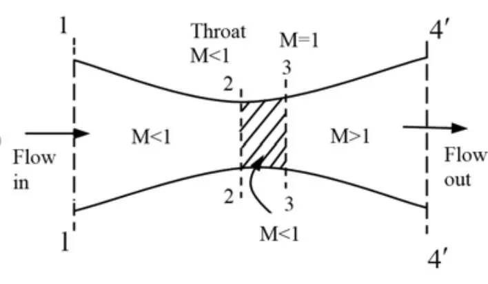
Mach number:
Mach number is a dimensionless quantity representing the ratio of flow velocity to speed of sound

where:
- M is the local Mach number,
- u is the local flow velocity
- c is the speed of sound in the medium
if M<1 = Subsonic flow
M>1 = Supersonic flow
M=1 = Sonic flow
Conservative & Non-conservative forms:
conservative form and Non conservative are mathematically equivalent they differ only in numerical discritization more accurate they tend to work when shock exists in domain
Conservative:
in conservative form control volume is stationary
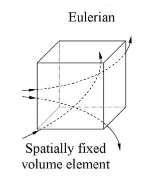
In Eulerian approach. we have a fixed point on space and we record the properties of fluid elements passing through it and we get conservative form of equation.
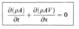
Continuity equation:
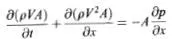
Momentum equation:
Energy equation:

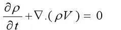
General form of continuity equation:
Non-Conservative:
in conservative form control volume is not stationary
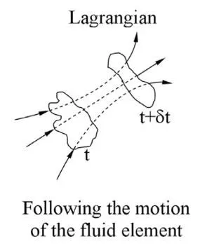
in lagrangian approach fluid particles travel through the flow we get non-conservative form of equation.
on doing non-dimenionalization of conservative forms we get
Continuity equation:
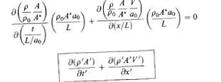
momentum equation:
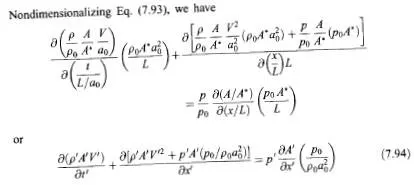

Energy equation:
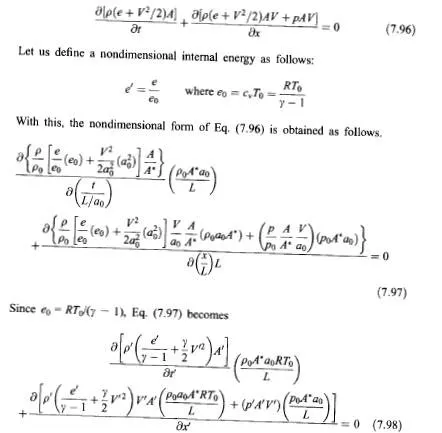
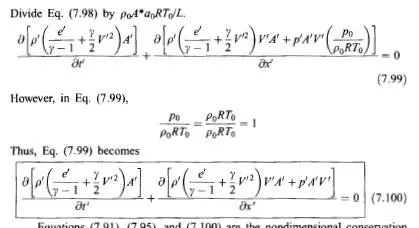
above equations are modified into simplest terms
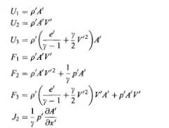
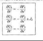
clear all
close all
clc
% inputs
n=31
x=linspace(0,3,n)
dx=x(2)-x(1)
gamma=1.4;
% caliculation of intial profile
rho=1-0.3146*x;
t=1-0.2314*x;
v=(0.1+1.09*x).*t.^0.5;
%area
a= 1+2.2*(x-1.5).^2;
%transpose(a)
%plot(a)
% Time step
nt=1400
dt=0.01;
% outer time loop
for k=1:nt
rho_old=rho;
v_old=v;
t_old=t;
%predictor method
for j=2:n-1
dvdx=(v(j+1)-v(j))/dx;
drhodx=(rho(j+1)-rho(j))/dx;
dtdx=(t(j+1)-t(j))/dx;
dlogadx=(log(a(j+1))-log(a(j)));
%continuity equation
drhodt_p(j)= -rho(j)*dvdx-rho(j)*v(j)*dlogadx-v(j)*drhodx;
%momentum equation
dvdt_p(j)=-v(j)*dvdx-(1/gamma)*(dtdx+(t(j)/rho(j))*drhodx);
%energy equation
dtdt_p(j)=-v(j)*dtdx-(gamma-1)*t(j)*(dvdx +v(j)*dlogadx);
% solution update
rho(j)=rho(j)+drhodt_p(j)*dt;
v(j)=v(j)+dvdt_p(j)*dt;
t(j)=t(j)+dtdt_p(j)*dt;
 end

%corrector method
for j=2:n-1
dvdx=(v(j)-v(j-1))/dx;
drhodx=(rho(j)-rho(j-1))/dx;
dtdx=(t(j)-t(j-1))/dx;
dlogadx=(log(a(j))-log(a(j-1)))/dx;
%continuity equation
drhodt_c(j)= -rho(j)*dvdx-rho(j)*v(j)*dlogadx-v(j)*drhodx;
%momentum equation
dvdt_c(j)=-v(j)*dvdx-(1/gamma)*(dtdx+(t(j)/rho(j))*drhodx);
%energy equation
dtdt_c(j)=-v(j)*dtdx-(gamma-1)*t(j)*(dvdx +v(j)*dlogadx);
end
%compute the average time derivative
drhodt=0.5*(drhodt_p+drhodt_c);
dvdt=0.5*(dvdt_p+dvdt_c);
dtdt=0.5*(dtdt_p+dtdt_c);
% Final solution update
for i=2:n-1
rho(i)=rho_old(i)+drhodt(i)*dt;
v(i)=v_old(i)+dvdt(i)*dt;
t(i)=t_old(i)+dtdt(i)*dt;
end
% apply boundary conditions
%inlet
v(1)=2*v(2)-v(3);
% outlet
v(n)=2*v(n-1)-v(n-2);
rho(n)= 2*rho(n-1)-rho(n-2);
t(n)= 2*t(n-1)-t(n-2);
end
M = v./sqrt(t);
m = rho.*a.*v;
p=rho.*t;

figure(1)
plot(x,p)
xlabel('x');
ylabel('Pressure')
title('Conservative presure');
%subplot(4,1,1)
hold on
figure(2);
plot(x,M);
xlabel('x');
ylabel('Mach number');
title('Machnumber');
%subplot(4,1,2)
hold on
figure(3)
plot(x,m)
title('Conservative mass');
xlabel('x');
ylabel('mass flow rate')
%subplot(4,1,3);
hold on
figure(4)
plot(x,t)
title('Temperature');
xlabel('x');
ylabel('Temperature ratios')
%subplot(4,1,4);
hold on
figure(5)
plot(x,rho)
title('Density');
xlabel('x');
ylabel('density ratios')
figure(6)
plot(x,v)
title('Velocity');
xlabel('x');
ylabel('Velocity ratios');
%% Non-conservative
clear all
close all
clc
% inputs
n=31;
x=linspace(0,3,n);
dx=x(2)-x(1);
gamma=1.4;
%area
a= 1+2.2*(x-1.5).^2;
% Time step
nt=1400;
dt=0.0267;
% caliculation of intial profile
for i=1:length(x)
  if x(i)>=0 && x(i)<0.5
  rho(i)=1;
  t(i)=1;
elseif x(i)>=0.5 && x(i)<1.5
  rho(i)=1-0.366*(x(i)-0.5);
  t(i)=1-0.167*(x(i)-0.5);
  elseif x(i)>=1.5&&x(i)<=3
  rho(i)=0.634-0.3879*(x(i)-1.5);
  t(i)=0.833-0.3507*(x(i)-1.5);
  end
end
V=0.59./(rho.*a);
% At Throat
U1=rho.*a;         % U=Solution vector
U2=rho.*a.*V;
U3=U1.*(t./(gamma-1)+(0.5*gamma*V.^2).*a);  %ERROR
% outer time loop
for k=1:nt
U1_old=U1;
U2_old=U2;
U3_old=U3;
F1=U2;
F2=(U2.^2)./U1+((gamma-1)/gamma)*(U3-0.5*gamma*(U2.^2)./U1);
%F3= gamma* U2.*U3./U1- 0.5* gamma*(gamma-1)*(U2.^3)./(U2.^2); error
F3= gamma* U2.*U3./U1- 0.5* gamma*(gamma-1)*(U2.^3)./(U1.^2);
%predictor method
for j=2:n-1
dF1dx=(F1(j+1)-F1(j))/dx;                       % F=Flux  vector
dF2dx=(F2(j+1)-F2(j))/dx;
dF3dx=(F3(j+1)-F3(j))/dx;
dadx=(a(j+1)-a(j))/dx;
J2=(1/gamma)*rho(j)*t(j)*dadx;                  % J= Source term
%Continuity equation
dU1dt_p(j)=-dF1dx;
%Momentum equation
dU2dt_p(j)=-dF2dx+J2;
%energy equation
dU3dt_p(j)=-dF3dx;
%intermediate update
U1(j)=U1(j)+dU1dt_p(j)*dt;
U2(j)=U2(j)+dU2dt_p(j)*dt;
U3(j)=U3(j)+dU3dt_p(j)*dt;
end
rho= U1./a;
V= U2./U1;
t=(gamma-1)*((U3./U1)-0.5*gamma*V.^2);
F1=U2;
F2=(U2.^2)./U1+((gamma-1)/gamma)*(U3-0.5*gamma*(U2.^2)./U1);
%F3= gamma* U2.*U3./U1- 0.5* gamma*(gamma-1)*(U2.^3)./(U2.^2); ERROR
F3= gamma* U2.*U3./U1- 0.5* gamma*(gamma-1)*(U2.^3)./(U1.^2);
%corrector method
for j=2:n-1
dF1dx=(F1(j)-F1(j-1))/dx;
dF2dx=(F2(j)-F2(j-1))/dx;
dF3dx=(F3(j)-F3(j-1))/dx;
dadx=(a(j)-a(j-1))/dx;
J2=(1/gamma)*rho(j)*t(j)*dadx;
% Continuity equation
dU1dt_c(j)=-dF1dx;
%  Momentum equation
dU2dt_c(j)=-dF2dx+J2;
%energy equation
dU3dt_c(j)=-dF3dx;
end
% Average of predictor and corrector step
dU1dt= 0.5*(dU1dt_p+ dU1dt_c);
dU2dt= 0.5*(dU2dt_p+ dU2dt_c);
dU3dt= 0.5*(dU3dt_p+ dU3dt_c);

  % Final solution update
for j=2:n-1
U1(j)=U1_old(j)+dU1dt(j)*dt;
U2(j)=U2_old(j)+dU2dt(j)*dt;
U3(j)=U3_old(j)+dU3dt(j)*dt;
end
% FINAL UPDATION OF rho,V,T REQUIRED BEFORE COMPUTING BC'S
rho= U1./a;
V= U2./U1;
t=(gamma-1)*((U3./U1)-0.5*gamma*V.^2);
% Boundary conditions
% Inlet
U1(1)=rho(1)*a(1);
U2(1)=2*U2(2)-U2(3);
U3(1)=U1(1)*((t(1)/(gamma-1))+(0.5*gamma*V(1)^2));
% outlet
U1(n)= 2*U1(n-1)-U1(n-2);
U2(n)= 2*U2(n-1)-U2(n-2);
U3(n)= 2*U3(n-1)-U3(n-2);
M = V./sqrt(t);
m = rho.*a.*V;
p=rho.*t;
rho_th(k) = rho(16);
t_th(k) = t(16);
p_th(k) = p(16);
V_th(k)  = V(16);
M_th(k) = M(16);
m_th(k) = m(16);
end

figure(1);
plot(x,M);
xlabel('x');
ylabel('Mach number');
title('Machnumber');
figure(2)
plot(x,m);
title('Conservative mass');
xlabel('x');
ylabel('mass flow rate')
figure(3)
plot(x,t);
title('Temperature');
xlabel('x');
ylabel('Temperature ratios')
figure(4)
plot(x,p)
xlabel('x');
ylabel('Pressure')
title('Conservative presure');
figure(5)
plot(x,rho)
title('Density');
xlabel('x');
ylabel('density ratios')
figure(6)
plot(x,V)
title('Velocity');
xlabel('x');
ylabel('Velocity ratios');

figure(7);
plot(M_th);
xlabel('time step');
ylabel('Timewise Mach number');
title('Machnumber');
figure(8)
plot(m_th);
title('Timewise Conservative mass');
xlabel('time step');
ylabel('mass flow rate')
figure(9)
plot(t_th);
title('Timewise Temperature');
xlabel('time step');
ylabel('Temperature ratios');
figure(10)
plot(p_th)
xlabel('x');
ylabel('Pressure')
title('Timewise Conservative presure');
figure(11)
plot(rho_th)
title('Density');
xlabel('time step');
ylabel('density ratios')
figure(12)
plot(V_th)
title('Timewise Velocity');
xlabel('time step');
ylabel('Velocity ratios')
Grid dependence test:
| rho/rho_t | T/T_t | P/P_t | Mach no | ||
|
n=31 |
non-cons | 0.639 | 0.836 | 0.534 | 0.998 |
| n=61 | non-cons | 0.638 | 0.835 | 0.532 | 1 |
|
n=31 |
cons | 0.652 | 0.841 | 0.548 | 0.978 |
| n=61 | cons | 0.639 | 0.835 | 0.534 | 1 |
1)density,pressure and temperature at intial and throat values are known
2) 2 grid points are considered n=31,61 for grid dependence test
3) with increase in grid points solution is more accurate
4) from results we can say non-conservative consumes less no of time
5) Non conservative can be easily programmed because they are in the form (p,v,t)
6) in conservative form,equations are expressed in flux variables and modified to solution vectors
7) Non conservative is more accurate because primitive values are easily solved
8) stability of problem is more in conservative compared to non-conservative because they remain constant accross shock or discontinuities