Week 7 - Simulation of a 1D Super-sonic nozzle flow simulation using Macormack Method

Aim : Simulation of 1D supersonic nozzle flow simulation using Macormack Method

Macormack's mathod:

The MacCormack method is a variation of the two step Lax Wendroff scheme but is much simpler in application. To illustrate the algorithm, consider the following first order hyperbolic equation

The application of MacCormack method to the above equation proceeds in two steps; a predictor step which is followed by a corrector step.

Predictor step: In the predictor step, a "provisional" value of at time level is estimated as follows

The above equation is obtained by replacing the spatial and temporal derivatives in the previous first order hyperbolic equation using forward difference

Corrector step: In the corrector step, the predicted value is corrected according to the equation

Note that the corrector step uses backward difference approximations for spatial derivative. The time-step used in the corrector step is in contrast to the used in the predictor step.

Replacing the term by the temporal average

to obtain the corrector step as

Problem Solution :

We consider the steady, isentropic flow through a convergent-divergent nozzle.The flow at the inlet to the nozzle comes from a reservoir.The flow expands isentropically to supersonic speeds at the nozzle exit, The flow is locally subsonic in the convergent section of the nozzle.

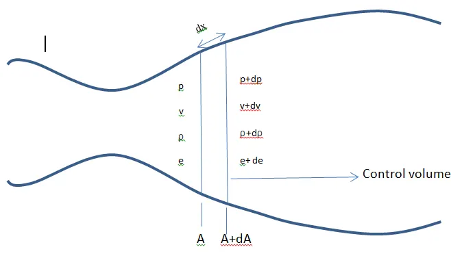
The flow field is two-dimensional (the flow varies in.the two-dimensional .ry space), we
make the assumption that the flow properties-vary only with x;assuming uniform flow properties across any given cross section. Such flow is defined as quasi-one-dimensional flow.The governing continuity, momentum, and energy equations for this quasione-dimensional, steady, isentropic flow can be expressed as

Continuity equation: ρ₁V₁A_{1 =} ρ₂V₂A₂

Momentum equation: P₁ A₁+ ρ₁ V₁² A₁ + ∫ PdA= P₂A₂ + ρ₂ V₂² A₂

Energy equation: h₁+ V₁²/2 = h₂+ V₂²/2

The above equations are solved in Conservative and Non conservative form of governing equations.

1) Non conservative form of governing equation:

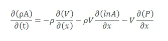
Continuity equation

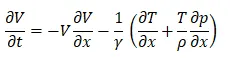
Momentum equation

Energy equation

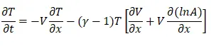
The above equation are Non dimensionalized non conservative from of govening equations. this equations are fruther solved by Macormack's mathod.The time step for the equation is calculated by using following formula

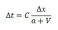
here, C is the Courant number the simple stability analysis of a
linear hyperbolic equation gives the result that C < l for an explicit numerical solution to be stable. The present application to subsonic supersonic isentropic nozzle flow is governed by nonlinear partial differential equations In this case, the exact stability criterion for a linear equation is that C <=1.

Boundary Conditions:

Subsonic inflow BC

V₁=2V₂-V₃

Supersonic outflow BC

V_N = 2V_N-1 - V_N-2

P_N = 2P_N-1 – P_N-2

T_N = 2T_N-1 - T_N-2

2) Conservative form of govening equation:

Continuity equation:

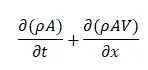
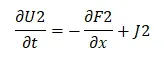
Momentum equation

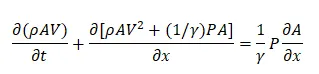
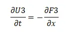
Energy equation

The above equation can be expressed in generic form. Let us define the elements of the solutions vector U, the flux vector F, and the source term J as follows.

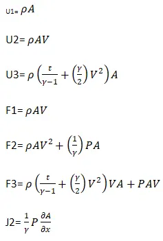
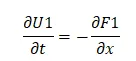
With this our general equations are written as

Continuity equation:

Momentum equation:

Energy euation:

Boundary condition:

Inlet boundary condition

u1(1)=rhoc(1)*a(1);
u2(1)=2*u2(2)-u2(3);
u3(1)=u1(1)*((tc(1)/(gamma-1))+((gamma/2)*vc(1)^2))

Outflow boundary condition:

u1(n)=2*u1(n-1)-u1(n-2);
u2(n)=2*u2(n-1)-u2(n-2);
u3(n)=2*u3(n-1)-u3(n-2);

Grid Spacing:

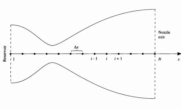
The first grid point, labeled point I, is assumed to be in the reservoir. The points are evenly distributed along the x axis, with dx denoting the spacing between grid points. The last point, namely, that at the nozzle exit, is denoted by N; we have a total number of N grid points distributed along the axis. Point i is simply an arbitrary grid point, with points i-1 and i+1 as the adjacent points.

Main Code:

n=31;
x=linspace(0,3,n);
dx=x(2)-x(1);
c=0.5
a=1+2.2*(x-1.5).^2;
throat=((n+1)/2);
%time steps
nt=1400;
gamma=1.4;
% non conservative from
[rho,v,t,m,p,M,rho_t,t_t,p_t,M_t]=non_cons(n,x,dx,c,a,throat,nt,gamma)

%conservative form
[rhoc,vc,tc,mc,pc,Mc,rhoc_t,tc_t,pc_t,Mc_t]=conservative(n,x,dx,c,a,throat,nt,gamma)

% plot Steady-state distribution of primitive variables inside the nozzle

%density
figure(3)
plot(x,rho)
hold on 
plot(x,rhoc,'*');
xlabel('length of Nozzle');
ylabel('Density');
legend('Non Conservative','Conservative');

%Temprature
figure(4)
plot(x,t)
hold on 
plot(x,tc,'*');
xlabel('length of Nozzle');
ylabel('Temprature');
legend('Non Conservative','Conservative');

%pressure
figure(5)
plot(x,p)
hold on 
plot(x,pc,'*');
xlabel('length of Nozzle');
ylabel('pressure');
legend('Non Conservative','Conservative');

%Mach number
figure(6)
plot(x,M)
hold on 
plot(x,Mc,'*');
xlabel('length of Nozzle');
ylabel('Mach number');
legend('Non Conservative','Conservative');

%Time wise variation of primitive variables
%Density
figure(7)
plot(1:nt,rho_t)
hold on 
plot(1:nt,rhoc_t)
xlabel('Time steps')
ylabel('density')
legend('Non Conservative','Conservative');

%Temprature
figure(8)
plot(1:nt,t_t)
hold on 
plot(1:nt,tc_t)
xlabel('Time steps')
ylabel('Temprature')
legend('Non Conservative','Conservative');

%pressure
figure(9)
plot(1:nt,p_t)
hold on 
plot(1:nt,pc_t)
xlabel('Time steps')
ylabel('Pressure')
legend('Non Conservative','Conservative');

%Mach number
figure(10)
plot(1:nt,M_t)
hold on 
plot(1:nt,Mc_t)
xlabel('Time steps')
ylabel('Mach number')
legend('Non Conservative','Conservative');

% plot Comparison of Normalized mass flow rate distributions of both forms
figure(11)
mexact=0.579*ones(1,31);
plot(x,m)
hold on 
plot(x,mc,'*')
hold on 
plot(x,mexact,'---')
xlabel('Length of nozzle')
ylabel('Mass flow rate')
legend('Non Conservative','Conservative','exact analytical value');

Function code for Non conservative equation:

function[rho,v,t,m,p,M,rho_t,t_t,p_t,M_t]=non_cons(n,x,dx,c,a,throat,nt,gamma)
%input
n=31;
x=linspace(0,3,n);
dx=x(2)-x(1);
c=0.5
%initial conditions
rho=1-0.3146*x;
t=1-0.2314*x; %t=temp
v=(0.1+1.09*x).*(t.^0.5);
%area
a=1+2.2*(x-1.5).^2;
throat=((n+1)/2);
%time steps
nt=1400;
dt=min(c*(dx./(sqrt(t)+v)))
%dt=0.001;
gamma=1.4;

%outer time loop
for k=1:nt
  %predictor methods
  k
  rho_old=rho;
  v_old=v;
  t_old=t;
  
  for j=2:n-1
  %drho_dt=-rho(j)*((v(j+1)-v(j))/dx)-rho(j)*v(j)*(log(a(j+1))-log(a(i)))/dx-v(j)*(rho(j+1)-rho(j))/dx
  dvdx=(v(j+1)-v(j))/dx;
  dadx=(log(a(j+1))-log(a(j)))/dx;
  drhodx=(rho(j+1)-rho(j))/dx;
  dtdx=(t(j+1)-t(j))/dx;
  %continuity equation
  
  drho_dtp(j)=-rho(j)*dvdx-rho(j)*v(j)*dadx-v(j)*drhodx;
  
  %ENERGY EQUATION
  dt_dtp(j)=-v(j)*(dtdx)-(gamma-1)*t(j)*(dvdx+v(j)*(dadx));
  
  %momentum equation
  dv_dtp(j)=-v(j)*(dvdx)-(1/gamma)*(dtdx+(t(j)/rho(j))*drhodx);
  
  %solution update
  v(j)=v(j)+dv_dtp(j)*dt;
  t(j)=t(j)+dt_dtp(j)*dt;
  rho(j)=rho(j)+drho_dtp(j)*dt;
  endfor
  %corrector step
  for j=2:n-1
  %drho_dt=-rho(j)*((v(j+1)-v(j))/dx)-rho(j)*v(j)*(log(a(j+1))-log(a(i)))/dx-v(j)*(rho(j+1)-rho(j))/dx
  dvdx=(v(j)-v(j-1))/dx;
  dadx=(log(a(j))-log(a(j-1)))/dx;
  drhodx=(rho(j)-rho(j-1))/dx;
  dtdx=(t(j)-t(j-1))/dx;
  %continuity equation
  drho_dtc(j)=-(rho(j)*dvdx)-rho(j)*v(j)*dadx-v(j)*drhodx;
  
  %ENERGY EQUATION
  dt_dtc(j)=-(v(j)*(dtdx))-(gamma-1)*t(j)*(dvdx+v(j)*(dadx));
  
  %momentum equation
  dv_dtc(j)=-(v(j)*(dvdx))-(1/gamma)*(dtdx+(t(j)/rho(j))*drhodx);
  
  endfor
  %compute the avg time derivative
  drho_dt=0.5*(drho_dtp+drho_dtc);
  dt_dt=0.5*(dt_dtp+dt_dtc);
  dv_dt=0.5*(dv_dtp+dv_dtc);
  %final solution update
  for i=2:n-1
    v(i)=v_old(i)+dv_dt(i)*dt;
    t(i)=t_old(i)+dt_dt(i)*dt;
    rho(i)=rho_old(i)+drho_dt(i)*dt;
  endfor
  %apply the boundary conditions
  %inlet
  v(1)=2*v(2)-v(3);
  %outlet
  v(n)=2*v(n-1)-v(n-2);
  rho(n)=2*rho(n-1)-rho(n-2);
  t(n)=2*t(n-1)-t(n-2);
  %mass flow rate
  m= rho.*a.*v;
  %non dimensional pressure
  p=rho.*t;
  %mach number
  M=v./sqrt(t);
  %analytical value of mass flow rate=0.579
  mexact=0.579*ones(1,31);
  % throat value0
  rho_t(k)=rho(throat);
  t_t(k)=t(throat);
  p_t(k)=p(throat);
  M_t(k)=M(throat);
  figure(1) 
    if k==50
    plot(x,m,'g')
    hold on 
    elseif k==100
    plot(x,m,'b')
    hold on 
    elseif k==150
    plot(x,m,'y')
    hold on 
    elseif k==200
    plot(x,m,'r')
    hold on 
    elseif k==700
    plot(x,m,'*')
    hold on 
    elseif k==1400
    plot(x,m,'o')
    hold on
    plot(x,mexact,'---')
    xlabel('length of nozzle')
    ylabel('mass flow rate')
    legend('50','100','150','200','700','1400','exact analytical solt')
    title('mass flow rate at differemt time steps (nonconservative)')
  endif
endfor
end

Function code for Conservative equation:

function[rhoc,vc,tc,mc,pc,Mc,rhoc_t,tc_t,pc_t,Mc_t]=conservative(n,x,dx,c,a,throat,nt,gamma)
% conservative form
l=3;
n=31;
x=linspace(0,3,n);
dx=x(2)-x(1);
a=1+2.2*(x-1.5).^2;
gamma=1.4;
c=0.5;
throat=((n+1)/2);

for i=1:n
  if (x(i)>=0 && x(i)<=0.5)
    rhoc(i)=1;
    tc(i)=1;
    elseif(x(i)>=0.5 && x(i)<=1.5)
    rhoc(i)=1-0.366*(x(i)-0.5);
    tc(i)=1-0.167*(x(i)-0.5);
    elseif(x(i)>=1.5 && x(i)<=3.5)
    rhoc(i)=0.634-0.3879*(x(i)-1.5);
    tc(i)=0.833-0.3507*(x(i)-1.5);
  end
end
vc=0.59./(rhoc.*a);
pr=rhoc.*tc;
u1=rhoc.*a;
u2=rhoc.*a.*vc;
u3=rhoc.*a.*((tc./(gamma-1))+((gamma/2).*(vc.^2)));
dt=min(c.*(dx./(sqrt(tc)+vc)));
nt=1400;

%outer time loop
for k=1:nt
   u1_old=u1;
   u2_old=u2;
   u3_old=u3;
  %flux terms
  f1=u2;
  f2=((u2.^2)./u1)+(((gamma-1)/gamma)*(u3-((gamma/2)*((u2.^2)./u1))));
  f3=((gamma*u2.*u3)./u1)-(gamma*(gamma-1)*(u2.^3))./(2*u1.^2);

  %predictor step
  for i=2:n-1
    
    df1dx(i)= (f1(i+1)-f1(i))/dx;
    df2dx(i)= (f2(i+1)-f2(i))/dx;
    df3dx(i)= (f3(i+1)-f3(i))/dx;
    
    dadx(i)=(a(i+1)-a(i))/dx;
    j2(i)=(1/gamma)*(rhoc(i)*tc(i))*dadx(i);
    %continuity
    du1dt_p(i)=-df1dx(i);
    %momentum
    du2dt_p(i)=-df2dx(i)+j2(i);
    %energy
    du3dt_p(i)=-df3dx(i);
    %solution updates
    u1(i)=u1(i)+du1dt_p(i)*dt;
    u2(i)=u2(i)+du2dt_p(i)*dt;
    u3(i)=u3(i)+du3dt_p(i)*dt;  
  endfor
  %decoding the value of rho,v,t after predictor step
  rhoc=u1./a;
  vc=u2./u1;
  tc=(gamma-1)*((u3./u1)-((gamma*vc.^2)/2));
  %updating flux 
  f1=u2;
  f2=((u2.^2)./u1)+(((gamma-1)/gamma)*(u3-((gamma/2)*((u2.^2)./u1))));
  f3=((gamma*u2.*u3)./u1)-(gamma*(gamma-1)*(u2.^3))./(2*u1.^2);
  %corrector step
  for i=2:n-1
    df1dx(i)=(f1(i)-f1(i-1))/dx;
    df2dx(i)=(f2(i)-f2(i-1))/dx;
    df3dx(i)=(f3(i)-f3(i-1))/dx;
    dlogadx(i)=(log(a(i))-log(a(i-1)))/dx;
   %update j2
   dadx(i)=(a(i)-a(i-1))/dx;
   j2(i)=(1/gamma)*(rhoc(i)*tc(i))*dadx(i);
  
   %continuity equt
    du1dt_c(i)=-df1dx(i);
    %momentum
    du2dt_c(i)=-df2dx(i)+j2(i);
    %energy
    du3dt_c(i)=-df3dx(i);
  end
  %avg 
  du1dt=0.5*(du1dt_p+du1dt_c);
  du2dt=0.5*(du2dt_p+du2dt_c);
  du3dt=0.5*(du3dt_p+du3dt_c);
%FINAL CALCULATION
  for i=2:n-1
    u1(i)=u1_old(i)+du1dt(i)*dt;
    u2(i)=u2_old(i)+du2dt(i)*dt;
    u3(i)=u3_old(i)+du3dt(i)*dt;
  end
  %apply inlet b.c
  u1(1)=rhoc(1)*a(1);
  u2(1)=2*u2(2)-u2(3);
  vc(1)=u2(1)/u1(1);
  u3(1)=u1(1)*((tc(1)/(gamma-1))+((gamma/2)*vc(1)^2));
  %outlet
  u1(n)=2*u1(n-1)-u1(n-2);
  u2(n)=2*u2(n-1)-u2(n-2);
  u3(n)=2*u3(n-1)-u3(n-2);
  %primitive variables(decoding)
  rhoc=u1./a;
  vc=u2./u1;
  tc=(gamma-1)*((u3./u1)-((gamma*vc.^2)/2));
  %mass flow rate
  mc=rhoc.*a.*vc;
  %pressure
  pc=rhoc.*tc;
  %mach no
  Mc=vc./sqrt(tc);
  %analytical value of mass flow rate=0.579
  mexact=0.579*ones(1,31);
  %throat values
  rhoc_t(k)=rhoc(throat);
  tc_t(k)=tc(throat);
  pc_t(k)=pc(throat);
  Mc_t(k)=Mc(throat);
  figure(2) 
    if k==50
    plot(x,mc,'g')
    hold on 
    elseif k==100
    plot(x,mc,'b')
    hold on 
    elseif k==150
    plot(x,mc,'y')
    hold on 
    elseif k==200
    plot(x,mc,'r')
    hold on 
    elseif k==700
    plot(x,mc,'*')
    hold on 
    elseif k==1400
    plot(x,mc,'o')
    hold on 
    plot(x,mexact,'---')
    xlabel('length of nozzle')
    ylabel('mass flow rate')
    legend('50','100','150','200','700','1400','exact analytical solt')
    title('mass flow rate at differemt time steps (conservative)')
  endif
  
end
end

Output:

1. Steady-state distribution of primitive variables inside the nozzle

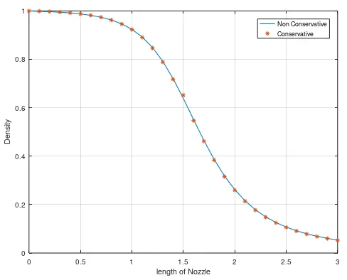
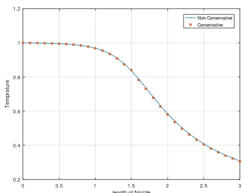
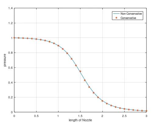
We have below plots for comparing values of Density Temperature, pressure and Mach number for Non consertive and conservative form of quasi-one-dimensional flow equations.

\

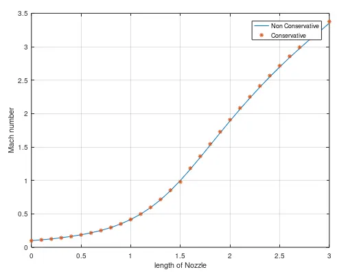
From the above plots we conclude that the values of both conservative and non conservative form of equations are the same as profiles matches for all the variables at no of grid points along the length of nozzle(x).

2. Time-wise variation of the primitive variables

The below plot shows variation of density, temperature, pressure and Mach number at the nozzle throat versus the number of time steps.

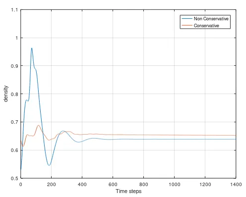
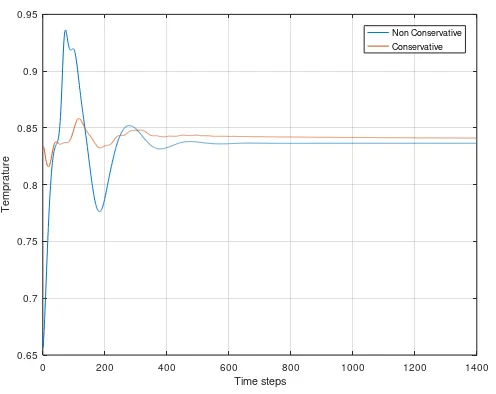
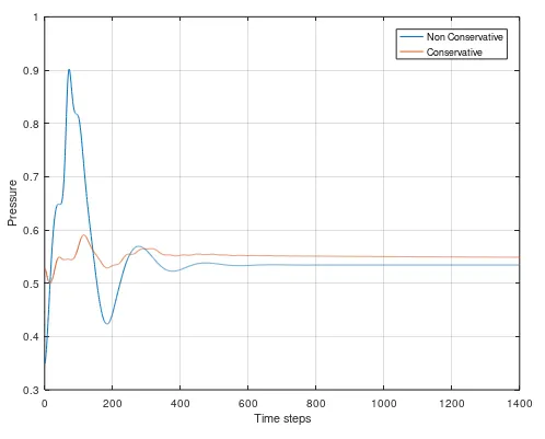
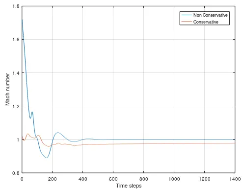
Total number of time steps are 1400 and we have made the following conclusion of variation of parameters at different timesteps.

1)Their is large amount of changes visible at early time steps i.e upto 200 timesteps we see their is rapid change in all the variables. this rapid changes are due to unstaedy compression and expansion of fluid initially propogating through nozzle.

2) As time steps increments along x-axis the staedy state flow is approached as flow variables becomes relaxed.the osscilation decreases between time steps 200 to 400.

3) we conclude that the staedy state is reached for both conservative and non conservative equations at minimum of 500 time steps. above which the equations converges to staedy state.

3. Variation of Mass flow rate distribution inside the nozzle at different time steps during the time-marching process

The below plots gives insight of the timewise variation of flow while it is approaching steady state considering the mass flow rate at no of time steps.

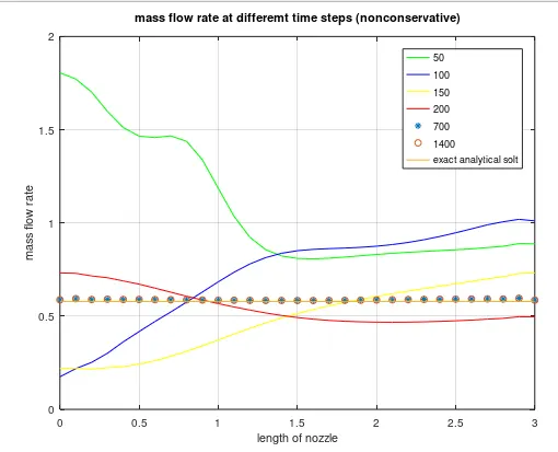
1) The curves shows variation of mass flow rate rho.a.v at different time steps along the length of nozzle(x). initially at 50 time steps the ditortion is on greater side as we have seen in time wise variation of different variables, the primitve variables shows oscillating changes in the plotwhich inturn effects the mass flow rate at initial time steps from 50 to 200 time steps.

2) this variation is accountable to transient variations of flow field variables. after 200 time steps the mass flow distribution begins to settle. after 700 time steps the mass flow rate is a straight line showm by blue*in above plot.it shows that mass flow is converged.

3) the variation of mass flow rate after 700 time steps is parallel to exact numerical value of mass flow rate shown in the plot.

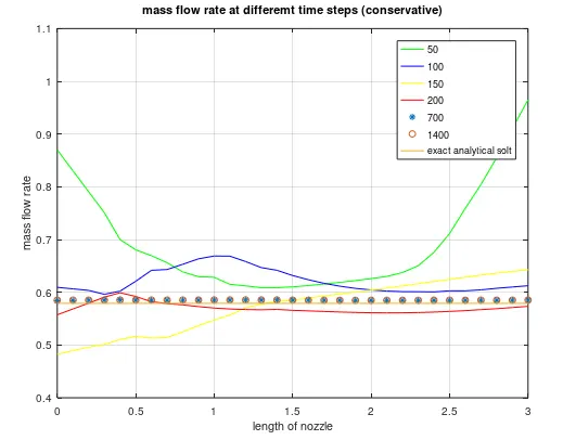
1) The above plot for conservative form of equation shows a straighth line for exact value of the equation solved numerically. the mass flow rate shows high deviation for initial time steps.

2) it shows that the mass flow rate is high initially as time derivative is large and as the time step increments the value of mass flow rate approches towards exact solution. after 700 time steps the value converges to steady state solution.

3) Their is similarity between plots for non conservative and conservative equation but as the boundary conditions are different for both equation they cannot be compared.

4. Comparison of Normalized mass flow rate distributions of both forms

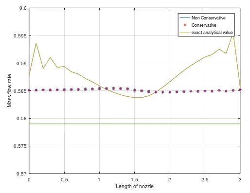
The steady-state variations of mass flow obtained with the nonconservation and conservation forms of the governing equations.This comparison is shown above in which the scale of the ordinate for mass flow is greatly magnified. Here we see that the steady-state mass flow distribution predicted by the conservation form of the equations is much more satisfactory than that obtained from the nonconservation form, on two accounts:

1. The conservation form gives a distribution that is much closer to being a constant. In contrast, the nonconservation results have (on the magnified scale) a sizeable variation, with some spurious oscillations at both the inflow and outflow boundries.

2. The steady-state mass flow results obtained with the conservation form are, on
the whole, much closer to the exact analytical solution of p'A'V' = 0.579, shown in above plot by the straigth line.

Grid Independence Test:

The above chart shows the grid independence test result done fo rboth conservative and non conservative equation. we have taken 31 and 61 numbers of grid points and throat values at i=16 and i=32.

The values obtained for density,temperature, pressure and Mach number clearly shows that increase in number of grid points gives more exact numerical values of the variables.

But the increase in no of grid points also increses the computational time and for larger number or complicated problems the cost of simulation will also increase with increase in computational memory and time.

Hence we conclude that increase in grid points gives marginally more accurate solution but at cost of incresed computational time and cost.

Conclusion:

From essence of all our previous discussion we come to following conclusion:

1) we can clearly say that primitive variable results obatained from non conservative form are more accurate than conservative form as shown in chart for 'grid independence test'.

2) but the mass flow rate obatined from conservative form is more close to the exact value of mass flow rate as we can see in ' Comparison of Normalized mass flow rate distributions of both forms'

3) No of calculation are more in conservative form as we have to decode the flux flux variables to find the primitive variables which is not the case for non conservative form.

4) The plots in 'Steady-state distribution of primitive variables inside the nozzle' shows that both the form of equations yields similar result for its primitive variables.