Week 9 - FVM Literature Review

The finite difference method (FDM) is not valid for more complex geometry as meshing is very complex or sometimes time consuming to be linear. hence we make use of more flexible method called Finite Volume Method (FVM).

The key step of the finite volume method is the integration of the transport equation over a three dimensional control volume (CV). At discrete places values are calculated on a meshed geometry.
The small volume which surrounds each node of the mesh is the grid cell.
In each grid cell, the volume integral of the divergence term is replaced by a surface integral, using
the Gauss divergence theorem. These terms are then evaluated as fluxes at the surfaces. This not
only ensures the conservation of fluxes entering and exiting the grid cell, but allows for easy
formulation of the balances on unstructured meshes.

Difference between FDM and FVM:

1) FDM is a differential scheme, that is approximation of a taylor series expansion. You try to write the first order, second order differential in terms of difference between two point values. This may bring in some approximation error.

let us consider one dimensional steady state heat conduction equation in a rod:

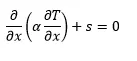
here α=thermal conductivity

s=source term

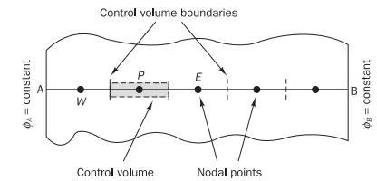
following is the representation of grid point distribution over volume of rod AB:

Step 1) Grid generation:

The first step in the finite volume method is to divide the domain into discrete control volumes. Let us place a number of nodal points in the space between A and B. The boundaries (or faces) of control volumes are positioned mid-way between adjacent nodes. Thus each node is surrounded by a control volume or cell. It is common practice to set up control volumes near the edge of the domain in such a way that the physical boundaries coincide with the control volume boundaries. At this point it is appropriate to establish a system of notation that can be used in future developments. now let us consider a nodal point P surrounded by two nodal points W AND E. the faces of the volume volume for node P is represented by e on est side and w on west side.The distances between the nodes W and P, and between nodes P and E, are identified by δxWP and δxPE respectively.the width of the control volume is delta x as shown in below fig.

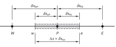
Step 2) Discritisation: In the case of finite volume method unlike fdm the governing equations are integrated over a control volume to obtain discritized equation at nodal point P.

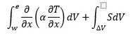
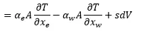
Here A is the cross-sectional area of the control volume face, ∆V is the volume and D is the average value of source S over the control volume. Equation above states that the diffusive flux of T leaving the east face minus the diffusive flux of T entering the west face is equal to the generation of T, i.e. it constitutes a balance equation for T over the control volume.

In order to derive useful forms of the discretised equations, the interface diffusion coefficient alpha and the gradient dα/dx at east (e) and west (w) are required. Following well-established practice, the values of T and the diffusion coefficient are defined and evaluated at nodal points.To calculate gradients (and hence fluxes) at the control volume faces an approximate distribution of properties between nodal points is used. Linear approximations seem to be the obvious and simplest way of calculating interface values and the gradients. This practice is called central differencing.In a uniform grid linearly interpolated values for αw and αe are given by

αw=αW+αP/2 αe=αP+αE/2

The diffusive term is written as

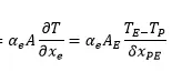(2)

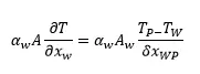(3)

In practical situations, as illustrated later, the source term S may be a function of the dependent variable. In such cases the finite volume method
approximates the source term by means of a linear form:
S∆V = Su + SpTP (4)

sunstituting equation 2,3 and 4 in equat 1

we get

(5)

Rearranging the above equation

(6)

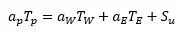
Identifying the coefficients of TW and TE in equation (6) as aW and aE, and
the coefficient of TP as aP, the above equation can be written as

(7)

where;

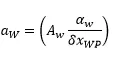
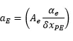
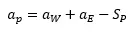
The values of Su and Sp can be obtained from the source model (4) S∆V = Su + SpTP. Equations 4 and 7 represent the discretised form of equation 1. This type of discretised equation is central to all further developments.

Step 3) Solution of the equation:

The discritized equation obtained in equation 7 must be setup at each nodal point to solve the equation. For control volumes that are adjacent to the domain boundaries the general discretised equation (7) is modified to incorporate boundary conditions. The resulting system of linear algebraic equations is then solved to obtain the distribution of the property T at nodal points.

Need for Interpolation schemes:

The appx of surface and volume integral may require values of variable at location other than nodes of control volume. the value are obtained in such cases using interpolation formulaes folowing are methods of interpolation:

1) central difference approximation

2) upwind difference approximation

3)Linear upwind difference scheme

4)quadratic upward differnce scheme (QUICK)

Need for Flux Limiters:

The task of the flux limiter is to determine an optimal value of each correction factor so as to remove as much artificial diffusion as possible without generating spurious oscillations.The main idea behind flux limiter is to realistic values.

For convective fluid flow in case of lower order scheme is usually stable but dissipative at the discountinous region. on the other hand the higher order schemes are unstable and shows oscillations in such discountinous regions. in such cases the flux limiters are used to tune the high order and low order scheme in such way that it gives higher order accuracy in smooth region nd first order accuracy in discountinuity region