Simple Pendulum

In Engineering, ODE is used to describe the transient behavior of a system. A simple example is a pendulum

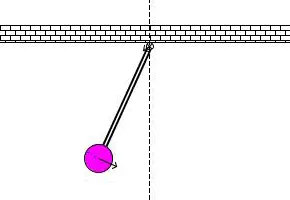
The way the pendulum moves depends on the Newtons second law. When this law is written down, we get a second order Ordinary Differential Equation that describes the position of the "ball" w.r.t time.

Similarly, there are hundreds of ODEs that describe key phenomena and if you have the ability to solve these equations then you will be able to simulate any of theses systems.

Your objective is to write a program that solves the following ODE. This ODE represents the equation of motion of a simple pendulum with damping.

Solution:

The ODE for simple pendulum considering damping is given as :

d2θdt2+(bm)⋅dθdt+(gl)⋅sin(θ)=0">d2θdt2+(bm)⋅dθdt+(gl)⋅sin(θ)=0d2θdt2+(bm)⋅dθdt+(gl)⋅sin(θ)=0

we cannot solve 2nd order ode in matlab hence we have to convert it into 1st order ode first and then perform the operation.

considering, θ=θ1(displacement)

dθ/dt=dθ1/dt=θ2(velocity)

d^2θ/dt^2=d^2θ1/dt^2=dθ2/dt

hence on substituting the above equation in our given ode

we get; dθ2/dt+(b/m)*θ2+(g/l)*sin(θ1)=0

we get a 2*1 matrix to solve for second order ode

y[dot1]=dθ1/dt=θ2

y[dot2]=dθ2/dt= -(b/m)*θ2+(g/l)*sin(θ1)

following is the main code

clear all
close all
clc
b=0.5;
m=1;
g=9.81;
l=1;
%initial conditions
t=[0;20];
theta0=[0;3]
%ode using anonymous function
[t theta]= ode45(@(t,theta) odefunc_pendulum(t,theta,b,m,g,l),t,theta0);
plot(t,theta(:,1))
hold on
plot(t,theta(:,2))
xlabel('t')
ylabel('angular velocity')
%animation and plotting
ct=1;
for i=1:length(theta(:,1));
  %origin
  x0=0;
  y0=0;
  %point at which bob is attached
  x1=l*sin(theta(i,1));
  y1=-l*cos(theta(i,1));
  %plot for pendulum
  plot([-1 1],[0 0],'linewidth',2,'color','k');
  %rope of pendulum from fixed origin to point of attachment of bob
  line([x0 x1],[y0 y1],'linewidth',2,'color','b');
  hold on;
  %to plot the bob using markers and facecolor
  plot(x1,y1,'-o','markers',20,'markerfacecolor','r');
  grid on;
  axis([-1.5 1.5 -1.5 0.5])
  pause(0.0003);
  hold off;
  %creating animation and saving it.
  printf('Creating GIF- Progress... %d/%d\n', i, length(t))
  img = print ('-RGBImage');
  imwrite(img, 'pendulumdamp.gif', 'DelayTime', .005, 'Compression', 'bzip', 'WriteMode', 'Append');
endfor

we have made use of function as we have 2 odes to solve hence we have not used only inbuilt function for ode45.following is the function:

function[ydot]=odefunc_pendulum(t,theta,b,m,g,l);
g=9.81;
%rateof change of displacement = velocity
ydot(1)=theta(2);
%angular acceleration 
ydot(2)= -(b/m)*theta(2)-(g/l)*sin(theta(1));
end

The plot between between time period(t) with respect to displacement and velocity shows the daming effect and change in magnitude of velocity and displacement as time t increases along x- axis.

We have created animation using inbuilt functions to keep track of image generated for each value of t and storing them the inbuilt function imwrite stores the images and then creates a animation.

Following is the animation:

link youtube video is below:

https://youtu.be/aZUT5EDGgBI