Simulation of a 1D Super-sonic nozzle flow simulation using Macormack Method
AIM
To simulate the isentropic flow through a quasi 1D subsonic-supersonic nozzle for conservative and non-conservative from of governing equations using MacCromack’s method.
THEORY
A convergent-divergent nozzle converts subsonic flow at inlet into supersonic flow at outlet.
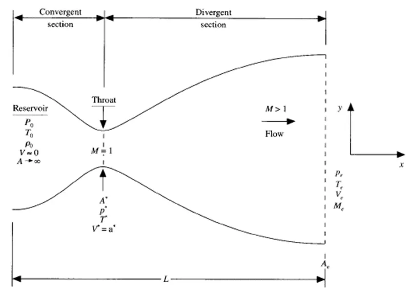
We consider a steady-isentropic flow through the nozzle shown above. The inlet flow comes from a reservoir and the cross-sectional are of the reservoir is large (theoretically it tends to infinity). For this problem, the flow varies in x and y direction, i.e., 2D flow. But we assume that flow property only varies on the x-axis. Such a flow is called quasi-one-dimensional flow.
The macCormack's technique is a predictor corrector method.
The governing equations can be written in non-conservative and conservation form. Non-dimensional form of these equations are used for simulation the flow. The non-dimensional variables are referenced to the reservoir values.
Non-conservative form
1. Continuity Equation
`(deltap^')/(deltat^') = -rho^'(deltaV^')/(deltax^')-rho^'V^'(delta(ln A^'))/(deltax^') - V^'(deltarho^')/(deltax^')`
2. Momentum equation
`(deltaV^')/(deltat^') = V^'(deltaV^')/(deltax^')-(1/gamma)((deltaT^')/(deltax^')+t^'/rho^'*(deltarho^')/(deltax^'))`
3. Energy equation
`(deltaT^')/(deltat^') = -V^'(deltaT^')/(deltax^') - (gamma-1)*T^'[(deltaV^')/(deltax^')+V^'(deltaln(A)^')/(deltax^')]`
Where,
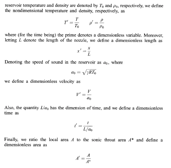
Using the MacCormack's approach,
In the predictor step, the governing equations are given as, , 


After the predictor step, we update the values of density, velocity and time,
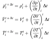
Now we go to corrector step. Here the governing equations are given as,

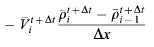



After the corrector steps, we find the average time derivates. They are found with the help of the following equations, 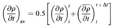
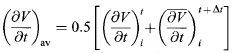
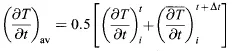
Then, we update the values of density, velocity, and temperature using the following equations
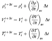
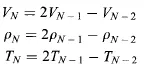
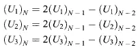
Lastly, we find the outflow boundary values.
Conservative Form (non-dimensional)
1. Contiunity Equation
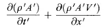

2. Momentum Equation

3. Energy Equation

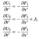
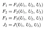
Consider U as solutiong vector, F as flux vetor and J as source term. Then,
Now, the conservative form of the governing equations become,
The flow variables are calculated as,
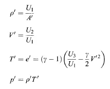
density, temperature and velocity is given by,
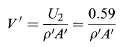
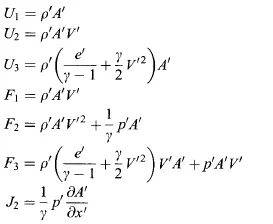
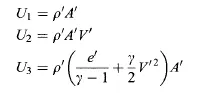
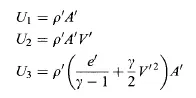
U1, U2, U3 are given as,
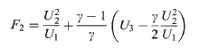
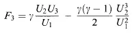
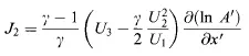
Flux and source term values in terms of U is given as,

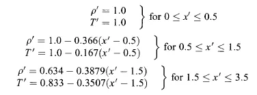
Initial conditions
Boundary conditions
CODE
1. Function code for non-conservative form
function [rho,v,t,mass_flow_rate,pressure,mach_no] = non_conservative_form(x,gamma,dx,n,nt,cfl)
        %calculate initial profiles
        rho = 1-0.3149*x; %density
        t = 1-0.2314*x; %temperature
        v = (0.1+1.09*x).*t.^0.5; %velocity
        %area
        a=1+2.2*(x-1.5).^2;
        %neck area
        neck = find(a==1);
        %timeloop
        for k=1:nt
            dt = min(cfl*dx./(sqrt(t)+v));

            rho_old = rho;
            v_old =v;
            t_old =t;

            %predictor method
            for j=2:n-1
                dvdx = (v(j+1)-v(j))/dx;
                drhodx = (rho(j+1)-rho(j))/dx;
                dtdx = (t(j+1)-t(j))/dx;
                dlogadx = (log(a(j+1))-log(a(j)))/dx ;
                %continuity
                drho_dt_p(j) = -rho(j)*dvdx - rho(j)*v(j)*dlogadx - v(j)*drhodx;
                %momentum
                dv_dt_p(j) = -v(j)*dvdx - (1/gamma)*(dtdx + (t(j)/rho(j))*drhodx);
                %energy
                dt_dt_p(j) = -v(j)*dtdx - (gamma-1)*t(j)*(dvdx + v(j)*dlogadx);

                %solution update
                rho(j) = rho(j) + drho_dt_p(j)*dt;
                v(j) = v(j) + dv_dt_p(j)*dt;
                t(j) = t(j) + dt_dt_p(j)*dt;
            end

            %corrector method
            for j=2:n-1
                dvdx = (v(j)-v(j-1))/dx;
                drhodx = (rho(j)-rho(j-1))/dx;
                dtdx = (t(j)-t(j-1))/dx;
                dlogadx = (log(a(j))-log(a(j-1)))/dx ;
                %continuity
                drho_dt_c(j) = -rho(j)*dvdx - rho(j)*v(j)*dlogadx - v(j)*drhodx;
                %momentum
                dv_dt_c(j) = -v(j)*dvdx - (1/gamma)*(dtdx + (t(j)/rho(j))*drhodx);
                %energy
                dt_dt_c(j) = -v(j)*dtdx - (gamma-1)*t(j)*(dvdx + v(j)*dlogadx);
            end

            %compute avg time derivative
            drhodt = 0.5*(drho_dt_p+drho_dt_c);
            dvdt = 0.5*(dv_dt_p+dv_dt_c);
            dtdt = 0.5*(dt_dt_p+dt_dt_c);

            %final solution update
            for m = 2:n-1
                rho(m) = rho_old(m) +drhodt(m)*dt;
                v(m)= v_old(m) + dvdt(m)*dt;
                t(m)= t_old(m) + dtdt(m)*dt;
            end

            %apply boundary conditions
            %inlet
            v(1) = 2*v(2)-v(3);
            %outlet
            v(n) = 2*v(n-1) - v(n-2);
            rho(n) = 2*rho(n-1) - rho(n-2);
            t(n) = 2*t(n-1) - t(n-2);

            %final mass flow rate
            mass_flow_rate = rho.*v.*a;
            %final pressures
            pressure = rho.*t;
            %final mach nos
            mach_no = v./sqrt(t);

            v_k(k)=v(neck);
            rho_k(k) = rho(neck);
            t_k(k) = t(neck);
            mass_flow_rate_k(k)=mass_flow_rate(neck);
            pressure_k(k)=pressure(neck);
            mach_no_k(k)=mach_no(neck);

            %comparing mass flow rates at different timesteps
            figure(1)
            if  k== 1
                plot(x,mass_flow_rate,'color','red','LineWidth',1);
                hold on
            elseif k==50
                plot(x,mass_flow_rate,'color','blue','LineWidth',1);
                hold on
            elseif k==100
                plot(x,mass_flow_rate,'color','green','LineWidth',1);
                hold on
            elseif k==200
                plot(x,mass_flow_rate,'color','magenta','LineWidth',1);
                hold on
            elseif k==400
                plot(x,mass_flow_rate,'color','cyan','LineWidth',1);
                hold on
            elseif k==800
                plot(x,mass_flow_rate,'color','black','LineWidth',1);
                hold on
            elseif k==1400
                plot(x,mass_flow_rate,'color','yellow','LineWidth',1);
                hold on
            end
            title('Mass flow rate of non conservative approach');
            xlabel('Length of the domain')
            ylabel('Mass Flow Rate')
            grid on
            legend('Mass Flow rate at timestep 1','Mass Flow rate at timestep 50','Mass Flow rate at timestep 100','Mass Flow rate at timestep 200','Mass Flow rate at timestep 400','Mass Flow rate at timestep 800','Mass Flow rate at timestep 1400');

        end
        %Time-wise variation of the primitive variables - non conservative
        figure(5)
        plot(rho_k,'color','red','LineWidth',1)
        hold on
        plot(v_k,'color','blue','LineWidth',1)
        plot(t_k,'color','green','LineWidth',1)
        plot(mach_no_k,'color','cyan','LineWidth',1)
        plot(mass_flow_rate_k,'color','magenta','LineWidth',1)
        plot(pressure_k,'color','black','LineWidth',1)
        title('Time-wise variation of the primitive variables - non conservative at the nozzle throat')
        legend('Desnity','Velocity','Temperature','Mach Number','Mass Flow Rate','Pressure')
        xlabel('Time Steps')
        ylabel('Primitive Values')
        grid on
end
2. Function code for conservative form
function [rho,v,t,mass_flow_rate,pressure,mach_no] = conservative_form(x,gamma,dx,n,nt,cfl)

        for k=1:n
            %density and temp values
            if (x(k)<=0.5)
                rho(k)=1;
                t(k)=1;
            elseif (x(k)>=0.5) && (x(k) <= 1.5)
                rho(k)=1-(0.366*(x(k)-0.5));
                t(k)=1-0.167*(x(k)-0.5);
            else
                rho(k)=0.634-0.3879*(x(k)-1.5);
                t(k)=0.833-0.3507*(x(k)-1.5);
            end
            %area
            a = 1+2.2*(x-1.5).^2;
            %velocity value
            v(k) = 0.59/(rho(k)*a(k));
        end

        %making copies or v, t, rho
        vold = v;
        told=t;
        rho_old=rho;
        %neck area
        throat = find(a==1);

        %initial solution vectors
        U1 = rho.*a;
        U2 = rho.*a.*v;
        U3 = rho.*((t./(gamma-1))+(gamma/2).*v.^2).*a;

        %mac cormack method
        %time loop
        for i=1:nt
            dt = min(cfl.*dx./(sqrt(t)+v)); %adaptive timestep
            %make copies of solution vector
            U1old=U1;
            U2old=U2;
            U3old=U3;

            F1 = U2;
            F2 = (U2.^2./U1)+((gamma-1)/gamma)*(U3-(0.5*gamma*U2.^2./U1));
            F3 = (gamma*U3.*(U2./U1))-((0.5*gamma*(gamma-1)).*(U2.^3)./(U1.^2));
            %predictor method
            for j=2:n-1
                %source term-J2
                J2(j)=(1/gamma)*rho(j)*t(j)*((a(j+1)-a(j))/dx);
                %contuinity eqn
                dU1_dt_p(j) = -((F1(j+1)-F1(j))/dx);
                %momentum eqn
                dU2_dt_p(j) = -((F2(j+1)-F2(j))/dx)+J2(j);
                %energy eqn
                dU3_dt_p(j) = -((F3(j+1)-F3(j))/dx);
                %updating solution vectors
                U1(j) = U1old(j)+dU1_dt_p(j)*dt;
                U2(j) = U2old(j)+dU2_dt_p(j)*dt;
                U3(j) = U3old(j)+dU3_dt_p(j)*dt;
            end

            %finding rho, v, and t from U1, U2, and U3
            rho = U1./a;
            v = U2./U1;
            t= (gamma-1).*((U3./U1)-(0.5*gamma.*v.^2));
            %updating flux vectors
            F1 = U2;
            F2 = (U2.^2./U1)+((gamma-1)/gamma)*(U3-(0.5*gamma.*U2.^2./U1));
            F3 = (gamma*U3.*U2./U1)-((0.5*gamma*(gamma-1)).*U2.^3./U1.^2);
            %Corrector Method
            for j=2:n-1
                %source term-J2
                J2(j)=(1/gamma)*rho(j)*t(j)*((a(j)-a(j-1))/dx);
                %contuinity eqn
                dU1_dt_c(j) = -((F1(j)-F1(j-1))/dx);
                %momentum eqn
                dU2_dt_c(j) = -((F2(j)-F2(j-1))/dx)+J2(j);
                %energy eqn
                dU3_dt_c(j) = -((F3(j)-F3(j-1))/dx);
            end
            %Computing avg time derivatives of solution vectors
            dU1_dt_avg = 0.5*(dU1_dt_p+dU1_dt_c);
            dU2_dt_avg = 0.5*(dU2_dt_p+dU2_dt_c);
            dU3_dt_avg = 0.5*(dU3_dt_p+dU3_dt_c);
            %Final Solution Update
            for m = 2:n-1
                U1(m) = U1old(m)+dU1_dt_avg(m)*dt;
                U2(m) = U2old(m)+dU2_dt_avg(m)*dt;
                U3(m) = U3old(m)+dU3_dt_avg(m)*dt;
            end
            %Inlet BC
            U1(1) = a(1);
            U2(1) = 2*U2(2)-U2(3);
            U3(1) = U1(1)*((t(1)/(gamma-1))+(0.5*gamma*(U2(1)/U1(1))^2));
            %Outlet BC
            U1(n) = 2*U1(n-1) - U1(n-2);
            U2(n) = 2*U2(n-1) - U2(n-2);
            U3(n) = 2*U3(n-1) - U3(n-2);
            %final values of rho,v,t
            rho = U1./a;
            v = U2./U1;
            t= (gamma-1).*((U3./U1)-(0.5*gamma.*v.^2));

            %final mass flow rate
            mass_flow_rate = rho.*v.*a;
            %final pressures
            pressure = rho.*t;
            %final mach nos
            mach_no = v./sqrt(t);

            rho_k(i)=rho(throat);
            v_k(i)=v(throat);
            t_k(i)=t(throat);
            mass_flow_rate_k(i)=mass_flow_rate(throat);
            pressure_k(i)=pressure(throat);
            mach_no_k(i)=mach_no(throat);


            %comparing mass flow rates at different timesteps
            figure(2)
            if  i== 1
                plot(x,mass_flow_rate,'color','red','LineWidth',1);
                hold on
            elseif i==50
                plot(x,mass_flow_rate,'color','blue','LineWidth',1);
                hold on
            elseif i==100
                plot(x,mass_flow_rate,'color','green','LineWidth',1);
                hold on
            elseif i==200
                plot(x,mass_flow_rate,'color','magenta','LineWidth',1);
                hold on
            elseif i==400
                plot(x,mass_flow_rate,'color','cyan','LineWidth',1);
                hold on
            elseif i==800
                plot(x,mass_flow_rate,'color','black','LineWidth',1);
                hold on
            elseif i==1400
                plot(x,mass_flow_rate,'color','yellow','LineWidth',1);
                hold on
            end
            title('Mass flow rate of conservative approach');
            xlabel('Length of the domain')
            ylabel('Mass Flow Rate')
            grid on
            legend('Mass Flow rate at timestep 1','Mass Flow rate at timestep 50','Mass Flow rate at timestep 100','Mass Flow rate at timestep 200','Mass Flow rate at timestep 400','Mass Flow rate at timestep 800','Mass Flow rate at timestep 1400');
        end
        %Time-wise variation of the primitive variables - conservative
        figure(6)
        plot(rho_k,'color','red','LineWidth',1)
        hold on
        plot(v_k,'color','blue','LineWidth',1)
        plot(t_k,'color','green','LineWidth',1')
        plot(mach_no_k,'color','cyan','LineWidth',1)
        plot(mass_flow_rate_k,'color','magenta','LineWidth',1)
        plot(pressure_k,'color','black','LineWidth',1)
        title('Time-wise variation of the primitive variables - conservative at the nozzle throat')
        legend('Desnity','Velocity','Temperature','Mach Number','Mass Flow Rate','Pressure')
        xlabel('Time Steps')
        ylabel('Primitive Values')
        grid on


end
3. Main code
clear all
close all
clc

%inputs
n = 31;
x =linspace(0,3,n);
dx = x(2)-x(1);
gamma = 1.4;
%timesteps
nt = 1400;
%courants number
cfl=0.5;

% calling non conservative function
tic
[rho_nc,v_nc,t_nc,mass_flow_rate_nc,pressure_nc,mach_no_nc] = non_conservative_form(x,gamma,dx,n,nt,cfl);
nc_time_31node = toc;
% calling conservative function
tic
[rho_c,v_c,t_c,mass_flow_rate_c,pressure_c,mach_no_c] = conservative_form(x,gamma,dx,n,nt,cfl);
c_time_31node = toc;


%plots
%steady state plot of primitive values - non conservative
figure(3)
plot(x,rho_nc,'color','red','LineWidth',1)
hold on
plot(x,v_nc,'color','blue','LineWidth',1)
plot(x,t_nc,'color','green','LineWidth',1)
plot(x,mach_no_nc,'color','cyan','LineWidth',1)
plot(x,mass_flow_rate_nc,'color','magenta','LineWidth',1)
plot(x,pressure_nc,'color','black','LineWidth',1)
title('Steady-state distribution of primitive variables inside the nozzle - non conservative  ')
legend('Desnity','Velocity','Temperature','Mach Number','Mass Flow Rate','Pressure')
xlabel('Length of the domain')
ylabel('Primitive Values')
grid on

%steady state plot of primitive values - conservative
figure(4)
plot(x,rho_c,'color','red','LineWidth',1)
hold on
plot(x,v_c,'color','blue','LineWidth',1)
plot(x,t_c,'color','green','LineWidth',1)
plot(x,mach_no_c,'color','cyan','LineWidth',1')
plot(x,mass_flow_rate_c,'color', 'magenta','LineWidth',1)
plot(x,pressure_c,'color','black','LineWidth',1)
title('Steady-state distribution of primitive variables inside the nozzle - conservative')
legend('Desnity','Velocity','Temperature','Mach Number','Mass Flow Rate','Pressure')
xlabel('Length of the domain')
ylabel('Primitive Values')
grid on

%normalized mass flow rates
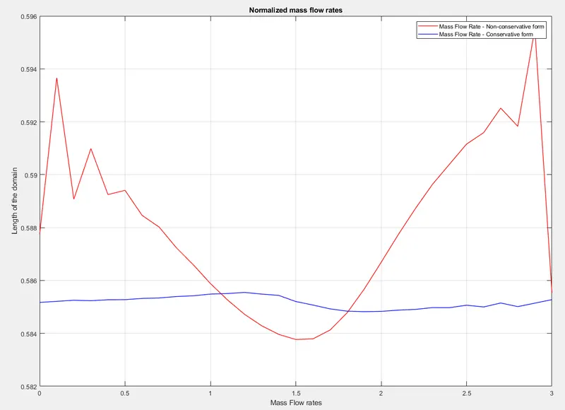
figure(7)
plot(x,mass_flow_rate_nc,'color','r','linewidth',1)
hold on
plot(x,mass_flow_rate_c,'color','blue','linewidth',1)
xlabel('Mass Flow rates')
ylabel('Length of the domain')
title('Normalized mass flow rates')
legend('Mass Flow Rate - Non-conservative form','Mass Flow Rate - Conservative form')
grid on
CODE EXPLAINATION
Function code:
In the function code, data which are common for both approaches are taken from the main code. In both cases, we have a predictor method. After this, we have solution update. After solution update, we have the corrector step. After this, we have final solution update. Then we find the initial and boundary conditions. This is run in a time loop of 1400 timesteps. This means it run for 1400 times.
Main Code:
Common data are created and then the respective functions are called. Then using data taken from the functions after they are executed, the required plots are created.
RESULTS AND CONCLUSION
1. NON CONSERVATIVE FORM
Mass Flow Rate
Primitive variables values inside the nozzle
Primitive variables at the throat of the nozzle at all timesteps
2. CONSERVATIVE FORM
Mass flow rate
Primitive variables values inside the nozzle
Primitive variables at the throat of the nozzle at all timesteps
3. Normalized mass flow rate
Grid Independence Test
This test tells us if our solution is dependent on the mesh. This means that change is mesh should not result in large/notable changes in our solution. When this happens, it means that out solution is grid independent. This test is carried out at 2 different mesh values. It is done at n=31 and n=61 and some values at the last node are taken for comparasion.
| Conservative approach | Non - Conservative approach | |||||
| n=31 | n=61 | Difference | n=31 | n=61 | Difference | |
| Velocity | 1.865912 | 1.863861 | 0.0020507 | 1.861787 | 1.863112 | -0.00132433 |
| Density | 0.052717 | 0.052563 | 0.0001541 | 0.052857 | 0.05265 | 0.000206893 |
| Temperature | 0.305479 | 0.307164 | -0.001685 | 0.308274 | 0.307893 | 0.000381504 |
| Time Taken | 89.74761 | 86.52621 | 3.2214072 | 90.2853 | 90.61938 | -0.3340774 |
Here in the above table, we can see that the difference is values at n=31 and n=61 are of negligible amount. This means that our soultion at n=31 is already grid independent.
CONCLUSIONS
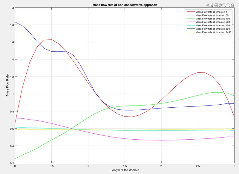
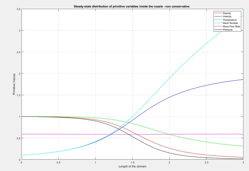
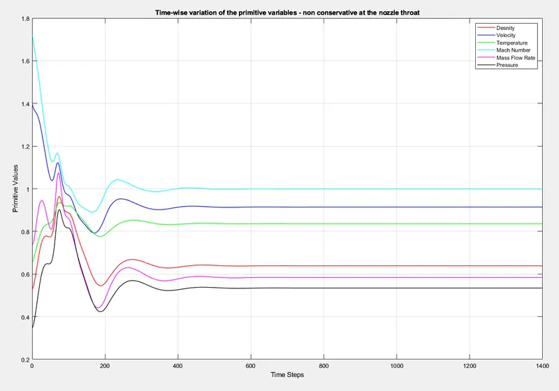
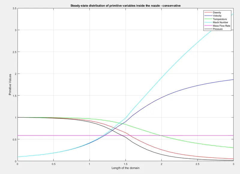
In the case of non-conservative approach, from the mass flow rate plot, we can see that between 400 and 800 timesteps, the mass flow rate is normalized and remains as such till 1400th timestep. The primitive variables values at the throat of the nozzel vary till approximately 600 timesteps and then remain unchanged. From the steady state plots, we can see that at the outlet, the mach no. is the highest. Similar characteristic is seen with velocity also. For density, temperature and pressure, the opposite is seen. They are at the lowest at the outlet.
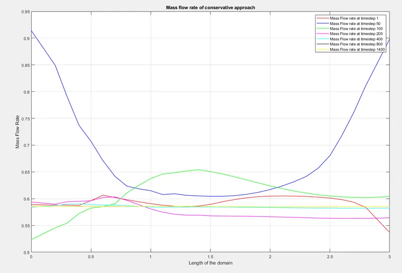
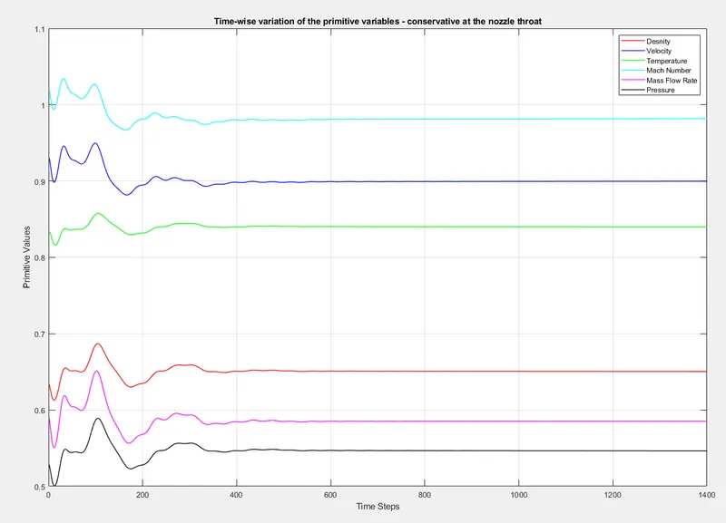
In conservative form, the majority of the characteristics are similar to the non-conservative form.
In the case of normalized mass flow rate comparision, the conservative approach looks to be more stable compared to the non conservative approach