Week 7 - Simulation of a 1D Super-sonic nozzle flow simulation using Macormack Method
SOLVING QUASI 1 - DIMENSIONAL SUPERSONIC NOZZLE FLOW EQUATION USING
MACCORMACK'S TECHNIQUE
AIM:
To Solve a Quasi 1-Dimensional supersonic nozzle flow equations using Maccormack's techniques for conservation and Non- conseration form of governing equations and also to analyze the temperature distribution for flow field variables.
OBJECTIVE:
- To solve Quasi 1-Dimensional subsonic- supersonic Nozzle flow equation.
- To derive Conservation and Non- conservation forms of governing equation for nozzle flow and solve by using Maccormack's techniques.
- To determine the steady state temperature distribution for flow field variables.
- To investigate the difference between conservation and Non-conservation forms of governing equations by comparing their solutions.
- To perform the grid indepence test on the solution in both conservation and Non conservation forms of governing equations.
PLOTTINGS:
- To Show the Steady-state distribution of primitive variables inside the nozzle.
- To Show the time-wise variation of the primitive variables.
- To show the Variation of Mass flow rate distribution inside the nozzle at different time steps during the time-marching process.
- To compare Normalized mass flow rate distributions of conservation and Non-conservation forms of governing equations.
INTRODUCTION:
DISCRETIZATION:
Discretization methods are used to divide the region of a continuous function i.e., the real solution to a system of differential equations into a discrete function, where the solution values are defined at each point in space and time. Discretization simply refers to the spacing between each point in solution space and then replace derivatives in the governing equation with difference quotients.
FINITE DIFFERENCE METHOD:
In numerical analysis, finite-difference methods (FDM) are a class of numerical techniques for solving differential equations by approximating derivatives with finite differences. Based on finite differences, it gives the numerical solutions for the values at discrete points in the domain which are known as grid points.
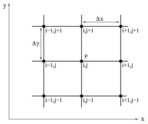
Finite differences method are used to compute approximate derivatives. This is used in numerical analysis in numerical ordinary differential equations and numerical partial differential equations, which gives the numerical solution of ordinary and partial differential equations respectively. The resulting methods are called finite-difference methods. Finite difference representations of derivatives are derived from Taylor series expansions.
MACORMACK'S TECHNIQUE:
The MacCormack method is a discretization scheme for the numerical solution of hyperbolic partial differential equations. This is a second-order finite difference method in both space and time. It consists of two steps namely predictor and corrector step by which the solutions are solved.
- The Predictor uses a forward difference scheme for spacial derivative.
- The corrector uses a backward difference scheme for spacial derivative.
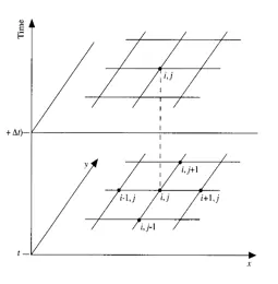
- In Maccormack's Mehthod the Average Mean time are determined between t and t + dt .
- The solutions are updated and the final primitive floe field variables are been determined.
It is a much simpler method compared to the other numerical methods which are dealing especially with the non-linear equations.
SUBSONIC - SUPER SONIC NOZZLE FLOW EQUATION:
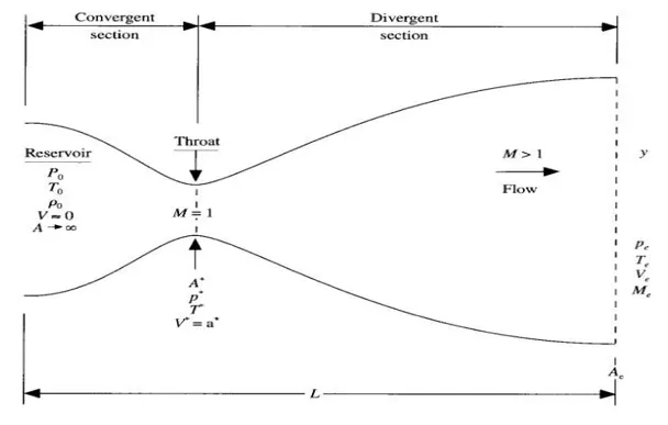
Considering a stedy, isentropic flow through a convergent Divergent Nozzle. The flow at the inlet of the nozzle comes from the reservoir where the pressure and temperature are denoted by `p_0` and `T_0` respectively.
The cross-sectional of the reservoir is very large A == `infty` and hence the velocity is very small (`V==0`). The flow expands isentropically at the supersonic speed at the exit, where the exit pressure, temperature, velocity, and Mach number are denoted by `p_e`, `T_e`, `V_e`, `M_e`.
The flow is subsonic (`M<1`) at the inlet of the nozzle, sonic at the throat section and super sonic at the outle(`M=1`).
DERIVING GOVERNING FLOW EQUATIONS
NON-CONSERVATION FORM:
In Non- Conservation form, Finite control volume fixed mass moving with the flow or infinitesimally small fluid element of fixed mass (fluid particle) moving with the flow. The Non-conservative equations are used for the moving system. That is why total derivative is used in non-conservative equations.
Considering Governig Partial Differential Equations for invisid flow (Euler Equation),
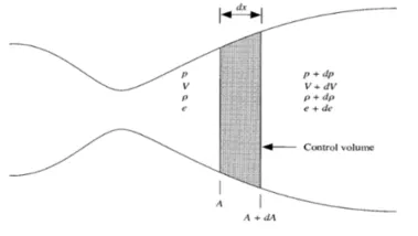
The integral form of the continuity equation is represented below,
`∂/(∂t)∫∫_V∫ρ∗dV+∫∫_Sρ∗v∗dS=0`
The equation is applied to the Shaded control volume. The left side of the figure consist of P, V rho and T and the right side oulets are represented by P+dp, V+dv, T+dt and `rho +drho`. They are uniform over the area A+da.
The partial differential Equation of Quasi one dimensional, general Non conservation form of equations,
- CONTINUTY EQUATION:
`(del (rho * A))/(delt) +(del (rho * A*v))/(delx)=0`
- MOMENTUM EQUATION:
`(rho(del * v))/(delt)+(rho*v*(del * v))/(delx)=- (delp)/(delx)`
- ENERGY EQUATION:
`(rho*c_v(del * T))/(delt) +(rho*V*c_v(del * T))/(delx)=- (rho*(del v))/(delx)-(rho* v*(del(logA))/(delx))`
NON DIMENSIONAL FORM OF EQUATIONS.
Using the Maccormack method using the Non dimensional form of governing equations to compute, The Non dimensional variables vary between 0 and 1.
- Non-dimensional temperature `T'=T/T_0`
`T_o` is the reservoir temperature
- Non-dimensional density `ρ'=ρ/ρ_0`
`ρ_o` is the reservoir density.
- Non-dimensional length `x'=x/L`
'L' is the nozzle length
- Non-dimensional velocity `v'=v/a_0`
a0 is the speed of the sound in the reservoir.
- Non-dimensional time `t'=t/(L/a_0)`
- Non-dimensional area `A'=A/(A∗)`
A∗ is the sonic throat area.
Replacing the above equation with non-dimensional variables we get,
GOVERNING EQUATIONS: (NON- DIMENSIONALIZED)
- CONTINUTY EQUATION :
`(∂ρ)/(∂t)=−ρ⋅(∂v)/(∂x)−ρ⋅v⋅(∂loga)/(∂x)−v⋅(∂ρ)/(∂x)`
- MOMENTUM EQUATION:
`(∂v)/(∂t)=−v⋅(∂v)/(∂x)−1/γ⋅((∂T)/(∂x)+T/ρ⋅(∂ρ)/(∂x))`
- ENERGY EQUATION:
`(∂T)/(∂t)=v⋅(∂T)/(∂x)−(γ−1)⋅[((∂v)/(∂x)+v⋅(∂(loga))/(∂x)]`
INITAL CONDITION FOR NON-CONSERVATION FORM,
Initial Conditions: @ time t=0,
Depending on the values of x-node we’re setting up the values for density, Velocity and Temperature in linear variation of flow field Variables,
Considering,
Density, `ρ=1−0.3146*x`
Velocity, `V=1-0.2314*x'
Temperature, `T=(0.1+1.09*x)T^(1/2)`
These are the linear variation of flow fiels variables as a function of x.
NOZZLE SHAPE,
- The throat area @ x = 1.5
- Convergence area of the nozzle are considered @ x<=1.5
- Divergence area of the Nozzle occurs @ X>=1.5
Assuming the Nozzle area to be Parabolic Area,
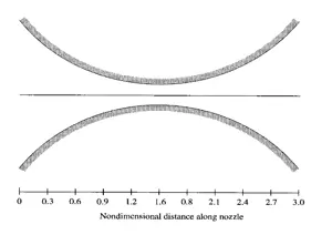
`A=1+2.2(x−1.5)^2 0<=X<=3`
MACH NUMBER,
Mach number (M) is a dimensionless quantity representing the ratio of flow velocity past a boundary to the local speed of sound.
`M= V/(√T)`
BOUNDARY CONDITIONS:
Subsonic Inflow Boundary: (@ Inlet),
Allowing one variable to float, Chossing the velocity V because on a physical basis as know that the mass flow through the nozzle must be allowed to adjust to the proper steady-state, and allowing other floe field variables are float at the outlets,
`V_1=2*V_2−V_3`
Density and temperature are fixed (independent of time),
`ρ_1=1 and T_1=1`
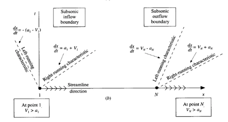
Supersonic Outflow Boundary: (@ End Node) ,
Allowing all flow-field variables to float:
`T_n=2*T_n−1−T_n−2`
`ρ_n=2*ρ_n−1−ρ_n−2`
`V_n=2*V_n−1−V_n−2`−V_n−2`
CONSERVATION FORM :
The conservative equation is applicable to the stationary system either fixed control volume fixed in space or infinitesimally small element fixed in space. If the solution is non-smooth, i.e., there are shocks, then the conservative equations should be used and discretized in a conservative way.
GOVERNING EQUATION:
- CONTINUTY EQUATION:
`(∂/(∂t)⋅ρ⋅a)=−(∂/(∂x)⋅ρ⋅a⋅v)`
- MOMENTUM EQUATION:
`(∂/(∂t)⋅ρ⋅a⋅v)+(∂/(∂x)[ρ⋅a⋅v^2+(1/γ)⋅ρ⋅a]=1/γ⋅ρ⋅(∂a)/(∂x)`
- ENERGY EQUATION:
`∂/(∂t)[ρ⋅(e/(γ−1)+(γ/2)⋅v^2)⋅a]+∂/(∂x)[ρ⋅(e/γ−1+(γ/2)⋅v^2)v⋅a+ρ⋅a⋅v]`
These equations are the non-dimensional conservative form of continuty, momentum and energy governing equations. These equations are quite unrealistic to see and hard to write the program with these.
So, need to write these in a generic form that can be easy and useful to write code. The conservative form of equation can be expressed in terms of solution vector U, Flux Vector F and Source Term J, the equations are devided into three parts as which are as follows,
- SOLUTION VECTOR,
`U_1=ρ⋅a`
`U_2=ρ⋅a⋅v`
`U_3=[ρ⋅(e/(γ−1)+(γ/2)⋅v^2)⋅a]`
- FLUX VECTOR,
`F_1=ρ⋅a⋅v`
`F_2=ρ⋅a⋅v^2+1/γ⋅ρ⋅a`
`F_3=[ρ⋅(e/(γ−1)+(γ/2)⋅v^2)v⋅a+ρ⋅a⋅v]`
- SOURCE TERM,
`J_2=1/γ⋅ρ⋅((∂a)/(∂x))`
The solution vector, Flux vector and source term are written in simplest form to form the Continuty, Momentum and Energy euqation of Conservative governing equations.
- CONTINUTY EQUATION,
`(∂U_1)/(∂t)=−(∂F_1)/(∂x)`
- MOMENTUM EQUATION,
`(∂U_2)/(∂t)=−(∂F_2)/(∂x)+J2`
- ENERGY EQUATION,
`(∂U_3)/(∂t)=−(∂F_3)/(∂x)`
These are the governing equations of the continuity, momentum and energy governing equations in conservative form of equations for 1 -Dimensional equation. From the solution vectores U(1,2,3) the primitive variables are determined. In the conservative form of governing equations, the dependent variables (the variables for which we directly obtain numbers) are not the primitive variables.
To obtain the primitive variables must decode the elements
`rho= U_1/A`
`V′=U_2/U_1`
`T′=e′=(γ−1)(U_3/U_1−γ/2(V′)^2)`
`P′=ρ′T′`
Therefore, after we obtain U1, U2 and U3 at each time step from the numerical solution of equations and the primitive variables are computed accordingly.
INITIAL CONDITION,
Initial Conditions: (@ TIME t=0)
For `0≤x′≤0.5`
`ρ′=1.0andT′=1.0`
For `0.5≤x′≤1.5:
`ρ′=1.0−0.366(x′−0.5)andT′=1.0−0.167(x′−0.5)`
For `1.5≤x′≤3.0:
`ρ′=0.634−0.3879(x′−1.5)andT′=0.833−0.3507(x′−1.5)`
For the initial condition only, let’s assume a constant mass flow through the nozzle and calculate V' as:
`V′=U_2/(ρ′A′)=0.59/(ρ′A′)`
The value of 0.59 is chosen for U2 because it is the closest to the exact analytical value of the steady-state mass flow (i.e. 0.579). Therefore, the initial condition for v' as a function of X' is obtained by substituting the variation.
Finally, the initial condition for U1, U2 and U3 are obtained by substituting the above variations for `ρ′,T',V'` into the definitions given for solution vector namely,
`U_1=ρ′A'`
`U_2=ρ′A'V`
`U_3=ρ′[(e′)/(γ−1)+γ/2(V′)^2]A'`
BOUNDARY CONDITIONS,
The boundary conditions for subsonic supersonic nozzle flow for conservation form of governing equations are subsonic inflow boundary with two properties with one float at inlet and all the flow properties are flot at outlet,
SUBSONIC INFLOW BOUNDARY: (@ Node 1)
Two properties are held fixed and one is allowed to float. `ρ'andT'` are fixed at inflow boundary, both equal to 1.0, and allowing `V'` to float:
`(U_1)_(i=1)=(ρ′A′)_(i=1)=A′_(i=1)=fixed value`
`(U_2)_(i=1)=2(U_2)_(i=2)−(U_2)_(i=3)`
`(U_3)_(i=1)=ρ′[(e′)/(γ−1)+γ/2V′^2]A'`
(or)
`(U_3)_(i=1)=U_1[(T′)/(γ−1)+γ/2V′^2]`
SUPERSONIC OUTFLOW BOUNDARY:(@ Node End),
All properties are allowed to float.
`(U_1)_N=2(U_1)_(N−1)−(U_1)_(N−1)`
`(U_2)_N=2(U_2)_(N−1)−(U_2)_(N−1)`
`(U_3)_N=2(U_3)_(N−1)−(U_3)_(N−1)`
CALCULATION OF TIME STEP,
For both non-conservative and conservative form of governing equations we’re going to take, time-step:
`Δt=C*Δx/(a+V)`
Where,
c =Courant number
v=local flow velocity
a =local speed of sound
For an explicit numerical solution to be stable:
`C≤1` (the simple stability analysis of a linear hyperbolic equation). For this particular problem, we’re taking, `c=0.5.`
The Courant-Friedrichs-Lewy (CFL) criterion for a one-dimensional flow, along with `C≤1`, it simply states that `Δt` must be less than, or at best equal to, the time taken by a sound wave to move from one grid point to the next.
`Δt = Miminum (Δt_1,Δt_2,........Δt_n)....`
STEPS INVOLVED IN PROGRAMMING:
STEP 1: Defining the input parameters for the domain for the Nozzle Flow.
STEP 2: Assuming the constant for specific heat and Courant number based on satbility.
STEP 3: Creating a function to solve conservation and Non conservation form of governing equations.
STEP 4: Deriving the equations for Conservation and Non-conservation form of governing equations.
STEP 6: Assuming the Initial and Boundary Conditions for Conservation and Non-conservation form of governing equations..
STEP7: Determining the Time step and Throat Position based on the grid points as a function of distance x.
STEP 8: Using the Maccormack's technique the governing form of equations are solved by predictor and corrector steps.
STEP 9: Updating the solutions and determining the Mach number and Mass flow distribution of primitive variables at different time steps.
STEP 10: Plotting the steady state distribution and Instataneous Mass flow distribution as a functio of distance and through the respective time steps.
STEP 12: Calling a function with respective forms of function name and comparing the solutions of Conservative and Non conservative forms of governig equations.
CODING:
M-CODE:
%% SOLVING QUASI 1-DIMENSIONAL SUBSONIC SUPERSONIC NOZZLE FLOW EQUATION
% Using Maccormack's Method to solve Conservation && Non-Conservation form of Governing Equations
close all;clc
%% Assigning the domain Parameters for Nozzle,
l=3;                 % Length of the Nozzle,
n=31;                % Number of Nodal Points [Considering Nodes as 31,61..]
x=linspace(0,l,n);   % Nozzle Length
dx=x(2)-x(1);        % Distance between grid points
%% Assuming the Constants,
gamma=1.4;            % For Air Constant
nt=1400;              % Number of time steps
c=0.5;                % Courant Number for stability condition
%% Calling a function,
% To solve Non-Conservative Form of Governing Equations by calling a function
[rho,t,v,M,p,mass_flow]=Non_conservation_sol(x,dx,n,nt,c,gamma);
% To solve Conservative Form of Governing Equations by calling a function
[rho_c,t_c,v_c,M_c,p_c,mass_flow_c]=conservation_sol(x,dx,n,nt,c,gamma);
%% Comparision of Normalized Mass Flow Rate Distribution of conservation and Non conservation
figure(7)
plot(x,mass_flow,'m','linewidth',1.25);   % Non conservative Normalized Mass Flow
hold on
plot(x,mass_flow_c,'g','linewidth',1.25); % Conservative Normalized Mass Flow
y = 0.579; % Exact analytical solution
line([0 3],[y y],'linewidth',1.25);
title('NORMALIZED MASS FLOW DISTRIBUTION');
subtitle('Conservation vs Non- Conservation vs Exact Solution')
legend('Non conservative','Conservative','Exact analytical solution','Location','north')
xlabel('x/L')
ylabel('Non dimensional mass flow (\rhoVA)/(\rho_{o}a_{o}A^{*})')
grid minor
FUNCTION FILE:
FUNCTION FILE FOR NON- CONSERVATION FORM OF GOVERNING EQUATION:
%% Creating a Function for Non conservation form of Governing Equation,
function [rho,t,v,M,p,mass_flow]=Non_conservation_sol(x,dx,n,nt,c,gamma)
%% Assuming the Non-Dimensional Initial Profiles Conditions,
a=1+2.2*(x-1.5).^2;   % Cross Sectional Area of the Nozzle
rho=1-0.3146*x;       % Initial Density
t=1-0.2314*x;         % Initial Temperature
v=(0.1+1.09.*x).*sqrt(t);  % Initial Velocity Profile
a_s=sqrt(t);          % Speed of sound
%% Calculation of Time step && Throat Position
dt=min(c*(dx./(a_s+v)));  % Time step
% Throat Position,        % A = A* at throat
n_throat = (n-1)/2;       % Throat is at 1.5m
%% Solving Non-Conservation form of Equation Using Maccormack's Technique
  for k=1:nt  % Time loop
    % Creating A copy of Density, Temperature and Pressure,
    rho_old=rho;
    t_old=t;
    v_old=v;
 %% (1). Predictor Step: (Using Forward Differencing Approximation)
    for i=2:n-1  % Loop for Inner Nodes,
       % Segregating & Expanding the terms,
        dv_dx=(v(i+1)-v(i))/dx;
        dlog_dx=(log(a(i+1))-log(a(i)))/dx;
        dr_dx=(rho(i+1)-rho(i))/dx;
        dt_dx=(t(i+1)-t(i))/dx;
     % Governing Equations,
         drho_dt_p(i)=-rho(i)*dv_dx-rho(i)*v(i)*dlog_dx-v(i)*dr_dx;    % Continuty Equation
         dv_dt_p(i)=-v(i)*dv_dx-(1/gamma)*(dt_dx+(t(i)/rho(i))*dr_dx); % Momentum Equation
         dt_dt_p(i)=-v(i)*dt_dx-(gamma-1)*t(i)*(dv_dx+v(i)*dlog_dx);   % Energy Equation
  %% (2) Solution Updating for flow field variables,
         v(i)=v(i)+dv_dt_p(i)*dt;        % Velocity
         t(i)=t(i)+dt_dt_p(i)*dt;        % Temperature
         rho(i)=rho(i)+drho_dt_p(i)*dt;  % Density
    end
   %% (3) Corrector Step: (Using Backward Differencing Approximation)
    for j=2:n-1
        % Segregating & Expanding the terms,
        dv_dx=(v(j)-v(j-1))/dx;
        dlog_dx=(log(a(j))-log(a(j-1)))/dx;
        dr_dx=(rho(j)-rho(j-1))/dx;
        dt_dx=(t(j)-t(j-1))/dx;
        % Governing Equations,
        drho_dt_c(j)=-rho(j)*dv_dx-rho(j)*v(j)*dlog_dx-v(j)*dr_dx;    % Continuty Equation
        dv_dt_c(j)=-v(j)*dv_dx-(1/gamma)*(dt_dx+(t(j)/rho(j))*dr_dx); % Momentum Equation
        dt_dt_c(j)=-v(j)*dt_dx-(gamma-1)*t(j)*(dv_dx+v(j)*dlog_dx);   % Energy Equation
    end
  %% (4) Computing Average Time Derivative,
       drho_dt=0.5*(drho_dt_p+drho_dt_c);   % Mean Desity Computing
       dv_dt=0.5*(dv_dt_p+dv_dt_c);         % Mean Velocity Computing
       dt_dt=0.5*(dt_dt_p+dt_dt_c);         % Mean Temperature Computing
   %% (5) Final Solution Update for floe field variables inside the nodel points,
        for m=2:n-1
          rho(m)=rho_old(m)+drho_dt(m)*dt; % Updating Density
          v(m)=v_old(m)+dv_dt(m)*dt;       % Updating Velocity
          t(m)=t_old(m)+dt_dt(m)*dt;       % Updating Temperature
        end
   %% (6) Applying Boundary Conditions,
      % Inflow Boundary Conditions
       v(1)=2*v(2)-v(3);           % @ Subsonic Inflow Boundary
      % Outflow Boundary Conditions
       v(n)=2*v(n-1)-v(n-2);       % @ Supersonic outlet Velocity
       rho(n)=2*rho(n-1)-rho(n-2); % @ Supersonic outlet Density
       t(n)=2*t(n-1)-t(n-2);       % @ Supersonic outlet Temperature
   %% Calculations For Mach Number, Pressure and Mass Flow Rate,
      % Mach Number,
      M=v./sqrt(t);    % Mach number
      % Pressure,
      p=rho.*t;        % Pressure (Non dimensional)
      % Mass Flow Rate,
      mass_flow=rho.*a.*v; % Mass flow rate (Non dimensional)
  %% Determining Nozzle Throat Area Flow field Variables,
      p_throat(k) = p(n_throat);     % Pressure
      rho_throat(k) = rho(n_throat); % Density
      T_throat(k) = t(n_throat);     % Temperature
      M_throat(k) = M(n_throat);     % Mach number
  %% Determining Mass Flow Rate Distribution @ Different time steps as a function of distance,
    figure(3)
    if (k == 1)
        plot(x,mass_flow,'--b')
        hold on
    elseif (k == 50)
        plot(x,mass_flow,'g','linewidth',1.25)
    elseif (k == 100)
        plot(x,mass_flow,'m','linewidth',1.25)
      elseif (k == 150)
        plot(x,mass_flow,'r','linewidth',1.25)
      elseif (k == 200)
        plot(x,mass_flow,'c','linewidth',1.25)
      elseif (k == 700)
        plot(x,mass_flow,'k','linewidth',1.25)
    title('Mass Flow Rate at Different Time Step (Non-Conservative Form)')
    xlabel('Distance(x)')
    ylabel('Mass Flow rate (\rhoVA)/(\rho_{o}a_{o}A^{*})')
    legend('0\Deltat','50\Deltat','100\Deltat','150\Deltat','200\Deltat','700\Deltat')
    grid minor
    end
  end
  %% PLOTTINGS
  % STEADY STATE DISTRIBUTION OF FLOW FIELD VARIABLES,
  figure(1)
   % Pressure Profile,
    subplot(4,1,1);
    plot(x,p,'r','LineWidth',1.1)
    title('Steady State Distribution For Quasi 1-Dimensional Flow Field Variables (Non-Conservative Form)')
    subtitle('Pressure Profile')
    ylabel('p/p_{o}')
    axis([0 3 0 1.2])
    legend('Pressure ratio')
    grid minor
   % Density Profile,
    subplot(4,1,2)
    plot(x,rho,'b','LineWidth',1.1)
    title('Density Profile')
    ylabel('\rho/\rho_{o}')
    axis([0 3 0 1.2])
    legend('Density ratio')
    grid minor
   % Temperature Profile,
    subplot(4,1,3)
    plot(x,t,'g','LineWidth',1.1)
    title('Temperature Profile')
    ylabel('T/T_{o}')
    axis([0 3 0 1.2])
    legend('Temperature ratio')
    grid minor
   % Mach Number,
    subplot(4,1,4)
    plot(x,M,'m','LineWidth',1.1)
    title('Mach Number')
    xlabel('Distance (x)')
    ylabel('Mach number')
    legend('Mach number','Location','best')
    axis([0 3 0 4])
    grid minor
%% Plotting Timewise Variation Of Priimitive Variables,
    figure(2)
   % Pressure @ Different Time steps as a function of Distance,
    subplot(4,1,1)
    plot(p_throat,'r','LineWidth',1.1)
    title('Time Wise Variation of Flow Field Variables (NON-CONSERVATIVE FORM)')
    subtitle('Pressure')
    ylabel('p/p_{o}')
    axis([0 1400 0.4 1.2])
    legend('Pressure')
    grid minor
   % Density @ Different Time steps as a function of Distance
    subplot(4,1,2);
    plot(rho_throat,'b','LineWidth',1.1)
    title('Density')
    ylabel('\rho/\rho_{o}')
    axis([0 1400 0.6 1.1])
    legend('Density')
    grid minor
   % Temperature @ Different Time steps as a function of Distance,
    subplot(4,1,3)
    plot(T_throat,'g','LineWidth',1.1)
    title('Temperature')
    ylabel('T/T_{o}')
    axis([0 1400 0.6 1.1])
    legend('Temperature')
    grid minor
   % Mach Number @ Different Time steps as a function of Distance,
    subplot(4,1,4)
    plot(M_throat,'m','LineWidth',1.1)
    title('Mach number')
    xlabel('Number of time steps(k)')
    ylabel('Mach number')
    axis([0 1400 0.5 1.5])
    legend('Mach Number')
    grid minor
FUNCTION FILE FOR CONSERVATION FORM OF GOVERNING EQUATION:
%% Creating a Function for conservation form of Governing Equation,
% Solving Using Maccormack's Technique
function [rho_c,T_c,v_c,M_c,p_c,mass_flow_c]=conservation_sol(x,dx,n,nt,c,gamma)
%% Assuming Non-Dimensional Initial conditions,
for i = 1:length(x)  % Creating Iteration @ Different Distance "x"
   if (x(i) >= 0 && x(i) < 0.5)          % Distance Between 0-0.5
      rho_c(i) = 1;
      T_c(i) = 1;
   elseif (x(i) >= 0.5 && x(i) < 1.5)    % Distance Between 0.5-1.5
       rho_c(i) = 1 - 0.366*(x(i) - 0.5);
       T_c(i) = 1 - 0.167*(x(i) - 0.5);
    elseif (x(i) >= 1.5 && x(i) <= 3)    % Distance Between 1.5-3
       rho_c(i) = 0.634 - 0.3879*(x(i) - 1.5);
       T_c(i) = 0.833 - 0.3507*(x(i) - 1.5);
   end
end
%% Considering Area of Nozzle as,
    A=1+2.2*(x-1.5).^2;   % Cross Sectional Area of the Nozzle
  %% Flow Field Variables,
    rho_c_old= rho_c;
    v_c = 0.59./(rho_c_old.*A);   % Analytical mass flow rate = 0.59
    p_c = rho_c_old.*T_c;         %  Non dimenisonal Pressure
    mass_flow_c_initial = rho_c_old.*A.*v_c;
  %% Initializing solution vectors,
    U1 = rho_c.*A;
    U2 = rho_c.*A.*v_c;
    U3 = rho_c.*A.*((T_c/(gamma - 1)) + ((gamma/2)*(v_c.^2)));
%% Calculation Of Time Step and Throat Position,
    a_c = sqrt(T_c);                  % Non dimensionalized speed of sound conservative Equation
    dt_c = min((c.*dx)./(a_c + v_c)); % Time step using CFL criteria
% Throat Position,    % A = A* at throat
   n_throat = (n-1)/2; % Throat is at 1.5m
%% Solving Conservation form of Equation Using Maccormack's Technique
  for k=1:nt  % Time loop
    % Creating A copy of Solution Vectors,
        U1_old = U1;
        U2_old = U2;
        U3_old = U3;
    %% Defininng the Flux Terms,
        F1 = U2;
        F2 = (U2.^2./U1) + ((gamma-1)/gamma)*(U3 - (gamma*U2.^2)./(2*U1));
        F3 = ((gamma*U2.*U3)./U1) - ((gamma*(gamma-1)/2)*(U2.^3./U1.^2));
%% (1). Predictor Step: (Using Forward Differencing Approximation,
     for i = 2:n-1  % Loop for inner nodes
        % Segregating & Expanding the terms,
        J2(i) = (1/gamma).*rho_c(i).*T_c(i).*((A(i+1)-A(i))/dx);
        dF1_dx = (F1(i+1) - F1(i))/dx;
        dF2_dx = (F2(i+1) - F2(i))/dx;
        dF3_dx = (F3(i+1) - F3(i))/dx;
       % Solution Vectors,
        dU1_dt_p(i) = - dF1_dx;
        dU2_dt_p(i) = - dF2_dx + J2(i);
        dU3_dt_p(i) = - dF3_dx;
  %% (2) Solution Updating,
        U1(i) = U1(i) + dU1_dt_p(i)*dt_c;
        U2(i) = U2(i) + dU2_dt_p(i)*dt_c;
        U3(i) = U3(i) + dU3_dt_p(i)*dt_c;
      end
      % Updating Flux Terms,
        F1 = U2;
        F2 = (U2.^2./U1) + ((gamma-1)/gamma)*(U3 - (gamma*U2.^2)./(2*U1));
        F3 = ((gamma*U2.*U3)./U1) - ((gamma*(gamma-1)/2)*(U2.^3./U1.^2));
      % Updating Primitive Variables,
        rho_c = U1./A;
        v_c = U2./U1;
        T_c = (gamma-1)*(U3./U1 -(gamma/2)*v_c.^2);
 %% (3) Corrector Step: (Using Backward Differencing Approximation)
    for i = 2:n-1 % Loop For Inner Nodes
      % Segregating & Expanding the terms,
        J2(i) = (1/gamma).*rho_c(i).*T_c(i).*((A(i)-A(i-1))/dx);
        dF1_dx = (F1(i) - F1(i-1))/dx;
        dF2_dx = (F2(i) - F2(i-1))/dx;
        dF3_dx = (F3(i) - F3(i-1))/dx;
      % Solution Vectors,
        dU1_dt_c(i) = - dF1_dx;
        dU2_dt_c(i) = - dF2_dx + J2(i);
        dU3_dt_c(i) = - dF3_dx;
    end
 %% (4) Computing Average Time Derivative,
        dU1_dt_avg = 0.5*(dU1_dt_p + dU1_dt_c);
        dU2_dt_avg = 0.5*(dU2_dt_p + dU2_dt_c);
        dU3_dt_avg = 0.5*(dU3_dt_p + dU3_dt_c);
 %% (5) Final Solution Update,
    for j = 2:n-1
        U1(j) = U1_old(j) + dU1_dt_avg(j)*dt_c;
        U2(j) = U2_old(j) + dU2_dt_avg(j)*dt_c;
        U3(j) = U3_old(j) + dU3_dt_avg(j)*dt_c;
    end
 %% (6) Applying Boundary Conditions,
    % Inflow Boundary Conditions
    U1(1) = rho_c(1)*A(1);    % rho = 1 at i = 1  % @ Subsonic Inflow Boundary
    U2(1) = 2*U2(2) - U2(3);
    U3(1) = U1(1).*(((T_c(1)/(gamma-1)) + ((gamma/2)*v_c(1).^2)));
    % Outflow Boundary Conditions
    U1(n) = 2*U1(n-1) - U1(n-2); % @ Supersonic outflow Boundary Condition
    U2(n) = 2*U2(n-1) - U2(n-2);
    U3(n) = 2*U3(n-1) - U3(n-2);
 %% Determining & Updating Primitive Variables,
    rho_c = U1./A;     % Conservative Density
    v_c = U2./U1;      % Conservative Velocity
    T_c = (gamma - 1)*((U3./U1) - ((gamma/2)*v_c.^2));  % Conservative Temperature
    p_c = rho_c.*T_c;  % Conservative Pressure
 %% Calculations For Mach Number and Mass Flow Rate,
    % Mach Number,
    M_c = v_c./sqrt(T_c);        % Mach number for conservation form
    % Mass Flow Rate,
    mass_flow_c = rho_c.*A.*v_c; % Mass flow rate (Non dimensional)
 %% Determining Nozzle Throat Area Flow field Variables,
    p_throat_c(k) = p_c(n_throat);     % Pressure
    rho_throat_c(k) = rho_c(n_throat); % Density
    T_throat_c(k) = T_c(n_throat);     % Temperature
    M_throat_c(k) = M_c(n_throat);     % Mach number
 %% Determining Mass Flow Rate Distribution @ Different time steps as a function of distance,
    figure(6)
    if (k == 1)
        plot(x,mass_flow_c_initial,'--b')
        hold on
    elseif (k == 100)
        plot(x,mass_flow_c,'m','linewidth',1.25)
      elseif (k == 200)
        plot(x,mass_flow_c,'c','linewidth',1.25)
      elseif (k == 700)
        plot(x,mass_flow_c,'k','linewidth',1.25)
    title('Mass Flow Rate at Different Time Step (Conservative Form)')
    xlabel('Distance(x)')
    ylabel('Mass Flow rate (\rhoVA)/(\rho_{o}a_{o}A^{*})')
    legend('0\Deltat','100\Deltat','200\Deltat','700\Deltat')
    ylim([0.5 0.7])
    grid minor
    end
  end
%% PLOTTINGS
  % STEADY STATE DISTRIBUTION OF FLOW FIELD VARIABLES,
   figure(4)
   % Pressure Profile,
    subplot(4,1,1);
    plot(x,p_c,'r','LineWidth',1.1)
    title('Steady State Distribution For Quasi 1-Dimensional Flow Field Variables (Conservative Form)')
    subtitle('Pressure Profile')
    ylabel('p/p_{o}')
    axis([0 3 0 1.2])
    legend('Pressure ratio')
    grid minor
   % Density Profile,
    subplot(4,1,2)
    plot(x,rho_c,'b','LineWidth',1.1)
    title('Density Profile')
    ylabel('\rho/\rho_{o}')
    axis([0 3 0 1.2])
    legend('Density ratio')
    grid minor
   % Temperature Profile,
    subplot(4,1,3)
    plot(x,T_c,'g','LineWidth',1.1)
    title('Temperature Profile')
    ylabel('T/T_{o}')
    axis([0 3 0 1.2])
    legend('Temperature ratio')
    grid minor
   % Mach Number,
    subplot(4,1,4)
    plot(x,M_c,'m','LineWidth',1.1)
    title('Mach Number')
    xlabel('Distance (x)')
    ylabel('Mach number')
    legend('Mach number','Location','best')
    axis([0 3 0 4])
    grid minor
    %% Plotting Time wise Variation Of Priimitive Variables,
    figure(5)
   % Pressure @ Different Time steps as a function of Distance,
    subplot(4,1,1)
    plot(p_throat_c,'r','LineWidth',1.1)
    title('Time Wise Variation of Flow Field Variables (Conservative Form)')
    subtitle('Pressure')
    ylabel('p/p_{o}')
    axis([0 1400 0.4 1.2])
    legend('Pressure')
    grid minor
   % Density @ Different Time steps as a function of Distance
    subplot(4,1,2);
    plot(rho_throat_c,'b','LineWidth',1.1)
    title('Density')
    ylabel('\rho/\rho_{o}')
    axis([0 1400 0.6 1.1])
    legend('Density')
    grid minorr a
   % Temperature @ Different Time steps as a function of Distance,
    subplot(4,1,3)
    plot(T_throat_c,'g','LineWidth',1.1)
    title('Temperature')
    ylabel('T/T_{o}')
    axis([0 1400 0.6 1.1])
    legend('Temperature')
    grid minor
   % Mach Number @ Different Time steps as a function of Distance,
    subplot(4,1,4)
    plot(M_throat_c,'m','LineWidth',1.1)
    title('Mach number')
    xlabel('Number of time steps(k)')
    ylabel('Mach number')
    axis([0 1400 0.5 1.5])
    legend('Mach Number')
    grid minor
CODING EXPLANATION:
- Inputting the Domain parameters for Nozzle.
- Assigning the number of nodes on x, based on the number of nodes the array for the x-axis are assigned to the length of the domain using linspace command, equal intervels of arrays are created over the domain length.
- Determining the distance between the two nodes dx, by differncing the second node to the first node.
`dx=x(2) -x(1) or dx=l/(nx-1)`
- Assuming the constants for the specific heat , Courant number for the stable solutions in explicit form of solving governing equations.
- The Courant Number for the explicit form of Maccormack's method are solved by considering CFL < 1.
- Creating a function to solve 1 Dimensional quasi subsonic supersonic nozzle flow equations using Conservation and Non conservation forms of governig equations.
- In the function, define the Inital condition for the nozzle at time t=0.
- By passing the inputs to the function the primitive variables are solved and computed respectively.
- The number of time steps are been assigned as 1400 times the iterations passes through to solve the Governing form equations.
- The Nozzle Throat positions are determined using,
`Throat = (n-1)/2`
- Using Maccormack's technique to solve conservative and Non-conservative form of governing equation.
- Initialize the time loop to number of steps to solve to attain steady state distribution of floe field variables.
- Using "for" loop to iterate the number of time steps to the internal nodes ndes repectively.
- Predictor method, In this step using Forward Differencing Approximation (FDA) the spacial derivative are numericlly discretized and analyzed.
- Updating the solutions of flow field variables with in the loop to iterrate through internal nodes of the nozzle at a distace specified.
- Corrector step, In this step, using Backward Differencing Approximations (BDA) the spacial derivatives are decretized and iterated through internal nodes of the nozzle using "for" loop.
- Computing the Average/ Mean value of the respective derivatives.
- Updating the final solutions by iterating through internal nodes of the Nozzle.
- Applying Boundary conditions at inflow and outflow.
- @ Inflow Boundary conditions allowing one primitive variable to float and others variables are independent of flow fields.
- @ Outflow Boundary Condition allowing all the variables to floating.
- After the assigning of Boundary conditions @ Inlet and @ outlet the Mach number are determined using local velocity to the speed of sound.
- Also, To determine the nozzle throat area flow field variables like Density, Pressure, Temperature and Mach number respectively.
- Instanteneous Mass floe distribution as a function of distance through a nozzle are detrmined @ different time steps (0,50,100,150,200,700..)
- Plotting the steady state distribution of flow field variables using subplot command.
- Plotting the Time wise variation of flow fiels variables at different time steps are plotted using subplot command.
- Calling a function with the respective function name for the computation of conservation and Non-conservation form of governing equations.
- Comparing the solutions of conservation and Non-conservation form of Governing eqautions of Normalized Mass flow rates and compare with the analytical solutions.
PLOTTING:
(1). PLOTTING FOR NON-CONSERVATION FORM FLOW FIELD VARIABLES
(i). STEADY STATE DISTRIBUTION OF PRIMITIVE VARIABLES,
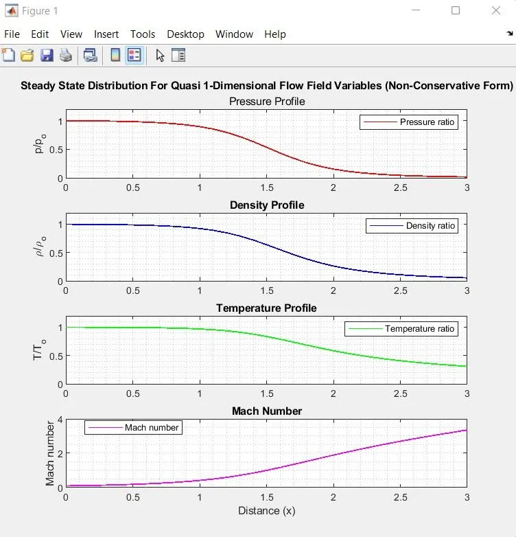
- The plotting describes the relationship between the Distance (x) as a function of Nozzle length through the number of nodal points represented to the primitive variables.
- The First subplot describes the Pressure Ratio of the Non conservation form of primitive flow field variable.
- The plots are descriptive between the values of 0 to 1 to represent the noticible range between the primitive flow fields.
- The second subplot describes the Density ratio of Non conservation form of primitive floe field variabel.
- Compared to the pressure and densiy the density of the flow field silghtly made differces at the outlet condition.
- The third subplot describe sthe Temperature ratio at the nozzle flow fields of Non conservation form of subsonic supersonic flows.
- The fourth subplot describes the Mach number of the flow through the nozzle initially at the inlet the mach number will be 0 then the primitive variables pressure, temperature and density flow on the nozzle increases the Mach number.
(ii). TIME - WISE VARIATION OF PRIMITIVE VARIABLES
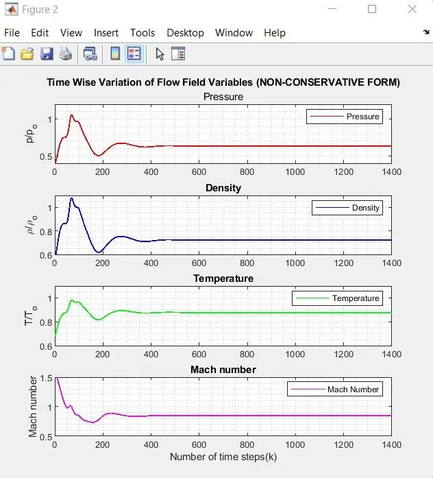
- The plotting describes the Time -Wise variation of flow fiels variables of density, ressure, temperature and Mach number at the Nozzle Throat.
- Based on the Number of time steps the Pressure, density, Temperature and Mach Number are been plotted.
- The largest changes occurs at the early stages of the nozzle flow.
- @ Earlier stage the flow field variables are osillated as much more and after the later stages the steady state is acheived itcomes to relaxation.
- The steady state condition are accomplished to maintain the linear variation in the flow field variables and the changes become smaller with respect to time.
- The oscillations are related to various expansion and compression stage progated in the nozzle during transient processm @ inlet flow condition.
(iii). MASS FLOW RATE DISTRIBUTION DIFFERENT TIME STEPS
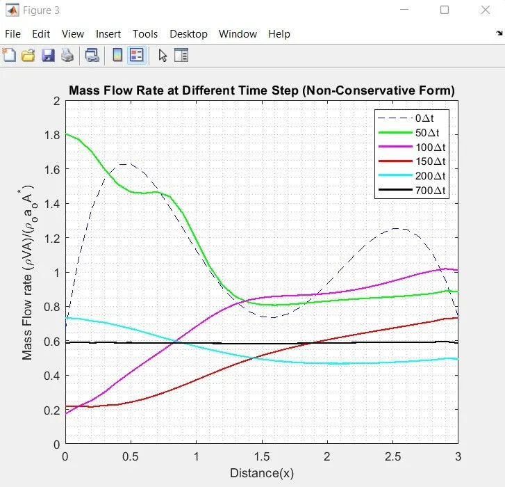
- The plotting describes the instanteneous Non dimensional mass flow distribution of as a function of distance through the nozzle at differnent time steps during time marchig approach.
- @ oΔt time step the mass flow rate shows th initila value sof velocity and density combained.
- @ 50Δt time step mass flow rate changes consideribely and @ 100Δ time step the mass flow rate changes radically and inside the nozzle the changes are radicallyy occured.
- @ 200Δt time step the mass flow rate settled doun slowly and @ 700Δt time step step it reaches the steady state condition of nozzzle flows.
- The Mass flow rate converges to constant and stady state throughout the nozzle.
(2). PLOTTING FOR CONSERVATION FORM FLOW FIELD VARIABLES
(i). STEADY STATE DISTRIBUTION OF PRIMITIVE VARIABLES,
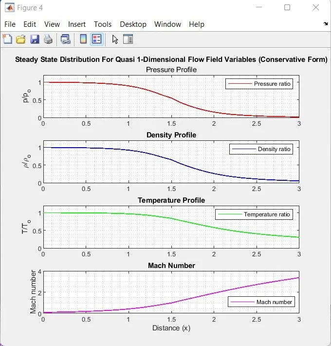
- The plotting describes the relationship between the Distance (x) as a function of Nozzle length through the number of nodal points represented to the primitive variables.
- The First subplot describes the Pressure Ratio of the conservation form of primitive flow field variable.
- The plots are descriptive between the values of 0 to 1 to represent the noticible range between the primitive flow fields.
- The second subplot describes the Density ratio of conservation form of primitive floe field variable.
- Compared to the pressure and densiy the density of the flow field silghtly made differces at the outlet condition.
- The third subplot describe sthe Temperature ratio at the nozzle flow fields of conservation form of subsonic supersonic flows.
- The fourth subplot describes the Mach number of the flow through the nozzle initially at the inlet the mach number will be 0 then the primitive variables pressure, temperature and density flow on the nozzle increases the Mach number.
(ii). TIME - WISE VARIATION OF PRIMITIVE VARIABLES
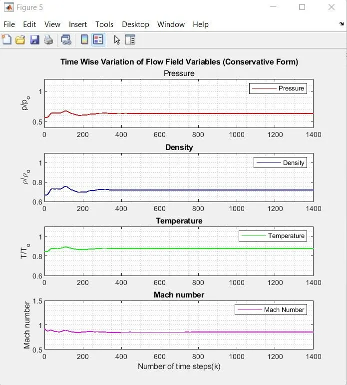
- The plotting describes the Time -Wise variation of flow fiels variables of density, ressure, temperature and Mach number at the Nozzle Throat.
- Based on the Number of time steps the Pressure, density, Temperature and Mach Number are been plotted.
- The largest changes occurs at the early stages of the nozzle flow.
- @ Earlier stage the flow field variables are osillated as much more and after the later stages the steady state is acheived itcomes to relaxation.
- The steady state condition are accomplished to maintain the linear variation in the flow field variables and the changes become smaller with respect to time.
- The oscillations are related to various expansion and compression stage progated in the nozzle during transient process.
(iii). MASS FLOW RATE DISTRIBUTION DIFFERENT TIME STEPS
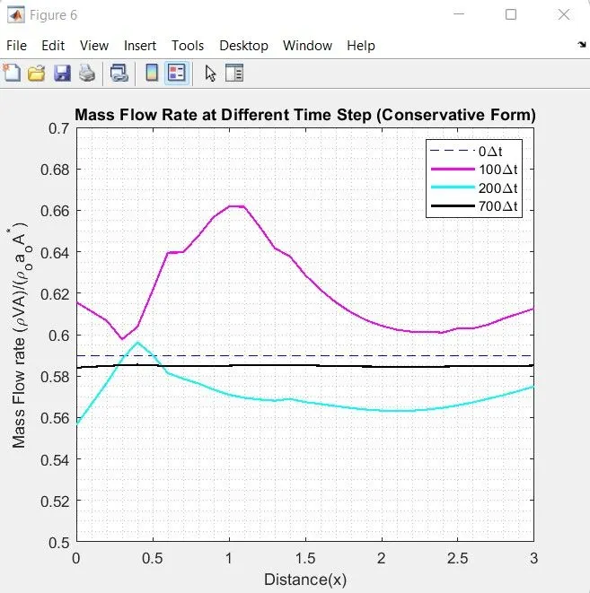
- The plotting describes the instanteneous Non dimensional mass flow distribution of mass floe rate as a function of distance through the nozzle at differnent time steps during time marchig approach.
- @ 0Δt time step the mass flow rate shows th initilay values of velocity and density combained.
- @ @ 100Δ time step the mass flow rate changes radically and inside the nozzle the changes are humped in a llarger variation occured.
- @ 200Δt time step the mass flow rate settled doun slowly and @ 700Δt time step step it reaches the steady state condition of nozzzle flows.
- The Mass flow rate converges to constant and stady state throughout the nozzle.
COMPARISION OF CONSERVATION AND NON- CONSERVATION SOLUTIONS,
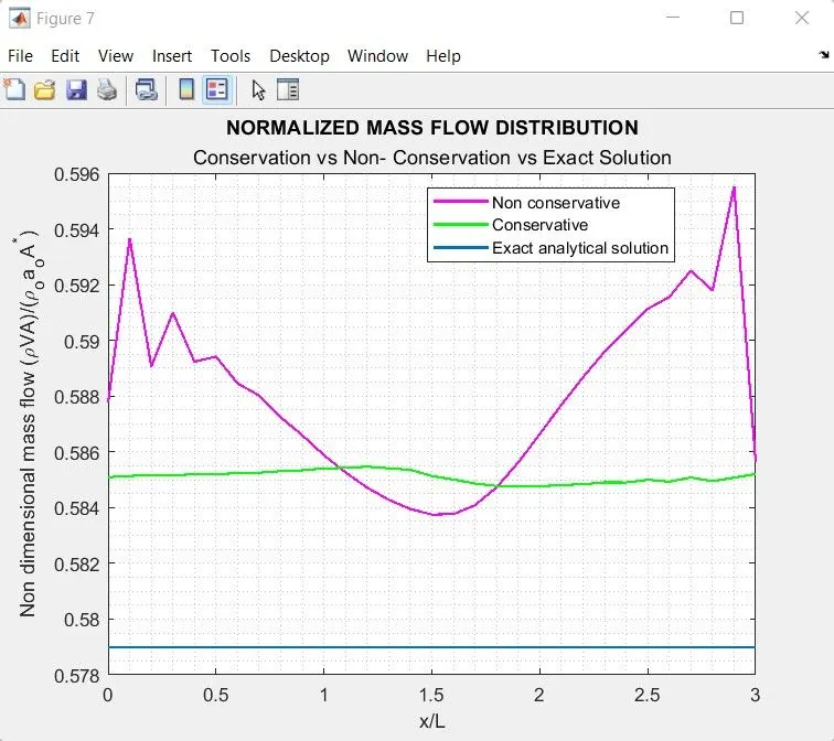
- The plotting compares the solution obtained from the mass floe rate of Conservation and Non conservation forms of governing equations @ time steps for 1400 time steps at a distance of nozzle x=3 through the nodel grid points n=31 and n=61.
- The conservation form gives the result likely to be constant. The Non conservation form gives initialy highly humed osicialltions dur to tranient at the infloe conditions.
- By comparing the conservation form with analytical form value sit will gives the better convergeence rate as compare with Non conervation form of governing equations.
- The conservation form preventing the mass throughout the flow field.
DOMENSTRATION OF GRID INDEPENDENCE TEST:
(1). NON CONSERVATION FORM
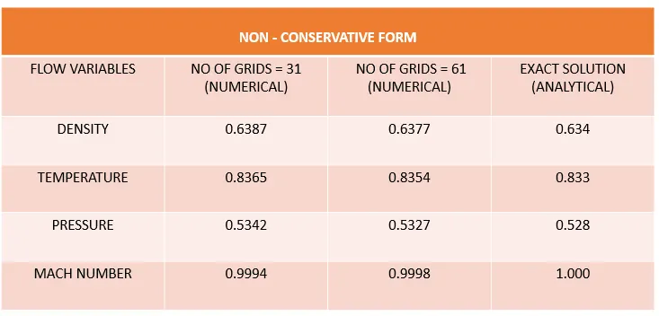
- The Tabulation of Non conservation form of flow field variable compares the density, temperature, pressure and Mach number at different grid sizes @ n=31 and n=61.
- Also, the exact analytical results are then compared with the ratio of density, pressure and temperature flow fields.
- By increasing the grid sizes from n-31 to n=61, will obsorb the change in the grid size inside the nozzle and also the results are comparatively equivalent with the exact solutions.
(2). CONSERVATION FORM
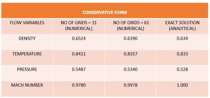
- The Tabulation of conservation form of flow field variable compares the density, temperature, pressure and Mach number at different grid sizes @ n=31 and n=61.
- Also, the exact analytical results are then compared with the ratio of density, pressure and temperature flow fields.
- By increasing the grid sizes from n-31 to n=61, will obsorb the change in the grid size inside the nozzle and also the results are comparatively equivalent with the exact solutions.
EFFECT OF COURANT NUMBER:
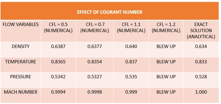
- The tabulation describes the effect of courant number and stability of the solution for bith conservation and Non conservation governing equations.
- The computations are made with the C=0.5, the solution are converged baed on thetime step and also the solution didn't blew up.
- Thesecelction of courant number is based on Courant-Friedrichs-Lewy (CFL) criterion for a one-dimensional flow, along with `C≤1`, it simply states that `Δt` must be less than, or at best equal to, the time taken by a sound wave to move from one grid point to the next.
- In the experimenatal analysis when increasing the CFL value from 0.5 to 1.2 the solution blew up occurs and instabilities occurs.
- In time marching procedure the selection of CFL will resembles in the stability of the solution.
OBSERVATIONS:
- The conservation form gives the better mass flow field distribution in conservating the mass through the nozzle as a function of nozzle distanec x.
- The residules in the conservation form are higher will results in the early times decays and later it will reach the steady state conditions.
- In Non conservation form of governing equations give sthe lesser residuls will resuts in the better flow field primitive variables.
- Comparing the results of conservative and Non conservation forms of governing equations, In Non conservative form of governing equations gives exact reault in the primitive avrialbes.
- In conservation form of Governing equations gives the sightly accurate results for the flux variables.
- In non conservation form to determinr the perimitive variables there is n need to decode the solution vectors.
- In conservation form of governing equations the decoding is need to findout the primitive varibles from the solution vectors.
M-CODE:
CONCLUSION:
- The Quasi 1-Dimensional subsonic- supersonic Nozzle flow equation are solved using Maccormack's Technique.
- The Conservation and Non- conservation forms of governing equation for nozzle flow equations are derived and analyzed using Maccormack's techniques.
- The steady state temperature distribution for flow field variables are determined.
- The difference between conservation and Non-conservation forms of governing equations by comparing their solutions are investigated and observed.
- The grid indepence test on the solution in both conservation and Non conservation forms of governing equations are been demonstrated.