SOLVING SECOND ORDER DIFFERENTIAL EQUATION USING MATLAB

AIM:

To write a Matlab program to solve second Order Differential Equation(ODE) .

OBJECTIVE:

To create an animation of a simple pendulum by solving ODE.

INTRODUCTION:

SIMPLE PENDULAM:

The pendulum is a simple mechanical system that follows a differential equation. The pendulum is initially at rest in a vertical position. When the pendulum is displaced by an angle θ and released, the force of gravity pulls it back towards its resting position. Its momentum causes it to overshoot and come to an angle −θ (if there are no frictional forces).

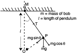
NOTATIONS:

Damping co-efficient= b

Acceleration due to gravity=g in (m/s^2)

Length of pendulum=l in (m)

Mass of the ball=m in (kg)

Angular displacement = d_0 in (rad)

Angular velocity= w_0 in (rad/s)

Initial condition =y_0

Counter=ct

STEPS INVOLVED IN PROGRAMMING:

STEP 1: Defining the inputs.

STEP 2: Creating a function for second order diffential equation

STEP 3: Assigning Initial conditions & Time intervals

STEP 4: Solving ODE

STEP 5: Plotting the results of Angular displacements and Angular velocity with respect to time

STEP 6: Assigning the counter to number of iterations

STEP7: Creating “For” loop to iterate the displacement to number of iteration ranges

STEP 8: Defining the co-ordinates.

STEP 9: Plotting the co-ordinates

STEP 10: Assign a counter for incremental iterations on loop.

STEP 11: Creating An Animation file for the plots of Simple pendulum

SECOND ORDER DEFFERENTIAL EQUATION:

This ODE represents the equation of motion of a simple pendulum with damping

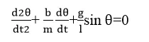.......(1)

Stepping down second order differential equation into first order by applying,

θ = θ1;

(dθ1/dt)= θ2; .......(2)

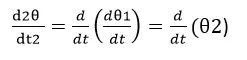.......(3)

By applying those conditions,substutuing equation (2) & (3) in equation (1)

(dθ2/dt)+(b/m)*(dθ1/dt)+(g/l)*sinθ1=0

(dθ2/dt)=-(b/m)*θ2-(g/l)*sinθ1

(d/dt)[θ1;θ2]=[θ2; -(b/m)*θ2-(g/l)*sinθ1]

Considering[θ1;θ2]=θ

(d/dt)θ=[θ2; -(b/m)*θ2-(g/l)*sinθ1] .........(solution)

CODING:

CREATING A FUNCTION TO SOLVE ODE

To create a function, apply the derived first order differential equation and by passing the inputs to function to solve the ODE.

%Creating a function to solve ODE

function [dtheta_dt]=ordinary_func(t,theta,b,m,g,l)

theta1=theta(1);
theta2=theta(2);
dtheta1_dt=theta(2);
dtheta2_dt=-(b/m)*theta(2)-(g/l)*theta(1);
dtheta_dt=[dtheta1_dt;dtheta2_dt];
end

CODING FOR SIMPLE PENDULUM:

%solving second order diffential equation (ODE)
%simple pendulum
clear all
close all
clc
%Inputs
b=0.05; %damping co-efficients
g=9.81; %Accelaretion due to gravity in (m/s^2)
l=1;    %Length of pendulum in (m)
m=1;    % Mass of ball in (kg)

%Initial conditions

d_0=0; %Angular displacement
w_0=3; %Angular velocity
y_0=[d_0;w_0]; %initial conditions for second order @t=0

%Time span 20 sec for pendulum oscillations

t_span=linspace(0,20,500); %initial time t_0=0 and t_f=20 with intervels 500

%solving ODE 

[t,solution]=ode45(@(t,theta)ordinary_func(t,theta,b,m,g,l),t_span,y_0);

%Plotting

figure(1) %Creates figure on separate window
plot(t,solution(:,1)); %To plot angular displacement
hold on % to add a second plot without deleting the existing plot
plot(t,solution(:,2)); %To plot angular velocity
axis([0 20 -4 4]); %setting the values for x & y axis
grid on
title('SIMPLE PENDULUM')
xlabel('Time (sec)');
ylabel('Angular Displacement (rad)/Angular Velocity (rad/s)');
legend('Angular Displacement','Angular Velocity') %To specify the plots
set(gca,'fontsize',14) %Properties will be added in plot

%To create Animation for simple pendulum

displacement=solution(:,1); %to create array for displacement
ct=1; %counter for incremental iterations on loop

for i=1:length(displacement) %loop created for number of iterations 
  angle=displacement(i); %the extracted displacements are stored in angle
  
 %Defining the co-ordinates
 %From the rigid support
   x0=0;
   y0=0;
 %from the length of pendulum
   x1=l*sin(angle);
   y1=-l*cos(angle);
   
%plotting for simple pendulum animation

figure(2) %Creates figure on separate window
plot([-1 1],[0 0],'linewidth',3) %plot line for rigid support
hold on  %to add a second  plot without deleting the existing plot

%Plotting the co-ordinates
plot([x0 x1],[y0 y1],'color','r','linewidth',3) 
plot(x1,y1,'o','markersize',20,'markerfacecolor',[1 0.5 0],'markeredgecolor',[1 1 1])
title('Oscillation Of A Simple Pendulum')
hold off %clear existing plots and reset all axes properties
grid on
axis([-1.2 1.2 -1.5 0.2]);
pause(0.01); %To pause for n seconds before continuing
M(ct)=getframe(gcf); %to get current figure with respect to counter
ct=ct+1; %incremental counter to each iterations in for loop

end
movie(M) %frames to play consecutively in the movie
videofile=VideoWriter('Transient Motion of a Simple Pendulum.avi','uncompressed AVI');
open(videofile) %open a certain videofile
writeVideo(videofile,M) %to write datas on file
close(videofile) %to close a file after writing

CODING EXPLANATION:

• Defining inputs for for mass, length ofpendulum, Acceleration due to gravity & Damping co-efficient
• Applying the initial conditions for angular displacement and angular velocity,
• Assigning the time span with equal intervels using linspace command
• Creating a function to solve ODE
• In order to solve ODE the second order differential equation is step down into first order differential equation which can solve by the "ode45"
• Solving ODE by using ode45
• Calling a function by the desired function name and passing the inputs to derive and integrate based on initial and time span conditions.
• To plot a solution after solving the second order diffential equation, angular displacements and angular velocity with respect to time are plotted.
• By using legend the angular displacement and angular velocity are identified in plot
• Then to ctreate an animation of the oscillation of simple pendulum
• In order to create an animation the displacements are arranged in an array to the number of iteration ranges.
• Ranges of displacements are iterated using the 'for' loop.
• The iterated values are been in angles to make displacements of pendulum
• Defining the co-ordinates in order to make a pendulum osscilations
• With the co-ordinates plotting are done.
• Creating the counter (ct) of increment to get frames of each loops and pause(n) command used to pause for n seconds before continuing on another loop.
• Animation is created by using the movie() command
• videowriter('') command is used to create a video file data on required video formats like .avi as used
• open() is used to open a certain videofile
• writevideo() is used to write datas on file
• close() is used to close a file after writing

PLOTTING:

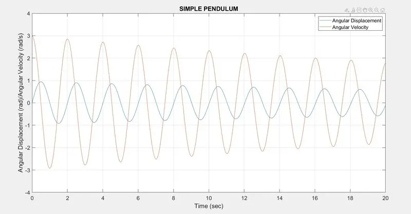
The plot describes the realtion between Angular displacementv(rad) with respect to time and Angular velocity (rad/s) with respect to time with damped oscillations of pendulum. The angular displacement and angular velocity of a simple pendulum also depends on mass and daming co-efficients.Due to the mass of ball that a state of equillibirium position to attain simple pendulum takes time with respect to damping co-efficient.

ERRORS FACED WHILE PROGRAMMING:

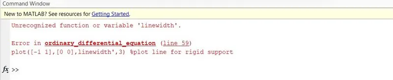
• Unrecognized variable error occured in plot proprties

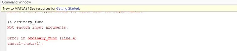
• While defining a functiom the input arrgument error occured

STEPS TAKEN TO OVERCOME THOSE ERRORS:

• In plot the properties are correctly assignied
• In function the input arguments are properly defined

VIDEO LINKS

1.https://youtu.be/272QLa7fZ-E

2.https://drive.google.com/file/d/1GPBb53XqJHt5T8Zu0cYoHlsJw32ziEpp/view?usp=sharing

CONCLUSION:

1. A Matlab program has been writtern to simulate motion of a simple pendulum
2. Solving ODE using ode45
3. Animation of swing of pendulum are created