OTTO CYCLE USING MATLAB CODE

AIM:

To write a matlab Program to solve an otto cycle(Air standared cycle)

OBJECTIVE:

1.To plot a PV diagram

2.To find the thermal efficiency of an engine

INTRODUCTION:

An Otto cycle is an idealized, Air standard thermodynamic cycle that describes the functioning of a typical spark ignition piston. The Otto cycle is a description of what happens to a mass of gas as it is subjected to changes of pressure, temperature, volume, addition of heat, and removal of heat. The mass of gas that is subjected to those changes is called the system. The system, in this case, is defined to be the fluid (gas) within the cylinder.

The Otto cycle is constructed from:

1. Isentropic (Adiabatic) Process(Compression & Expansion)

2. Constant Volume (Heat addition & Heat rejection)

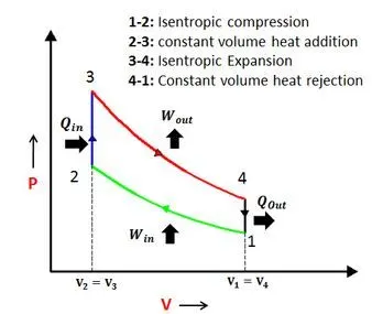
PROCESS IN OTTO CYCLE:

Process 1 – 2: Isentropic Compression

• This process is also known as the Compression Stroke, wherein the piston of the cylinder compresses the mixture of air and the fuel.

Process 2 – 3: Constant volume heat addition

• This process is also known as the Power Stroke, wherein the spark plug of the engine ignites the compressed mixture of air and fuel.

Process 3 – 4: Isentropic Expansion

• This process is also known as the Exhaust Stroke wherein the piston of the engine pushes the cylinder up thereby releasing the burned gases.

Process 4 – 1: Constant volume heat Rejection

• This process is also known as the Intake Stroke wherein the piston of the cylinder moves down the cylinder thereby resulting to an intake of air.

NOTATIONS:

• Temperature=t in (k)
• Volume=v in (m³)
• Pressure=p in (pascal)
• Crank pin radius=a in (m)
• Swept_volume=v_s in (m^3)
• clearence_volume=v_c in (m^3)
• Compression ratio=cr
• Specific heat ratio=gamma
• Ratio of connecting rod to crank pin radius=R

STEPS INVOLVED IN PROGRAMMING:

STEP 1: Defining Inputs for initial pressure & temperature, peak temperature, compression ratio, specific heat ratio.

STEP 2: Defining inputs to Engine Geometric parameters.

STEP 3: Calculate the state points of an otto cycle

STEP 4: Creating a Function to calculate Volume trace

STEP 5: Calling a function to define Compression and expansion for pressure and volume respectively.

STEP 6: Plotting the state points for PV Diagram

STEP 7: Calculate Thermal Efficiency of an engine.

CODING FOR STATE POINTS:

%Air standared cycle:
%There are 4 states 
clear all
close all
clc
% Consider Inputs
p1=110185; %initial pressure in (pascal)
t1=400; %initial temperature in (kelvin)
t3=2100; %peak temperature in (kelvin)
cr=10; %compression ratio
gamma=1.4; %specific heat ratio(cp/cv)

%Engine geometric parameters:
bore=0.12; %bore diameter in(m)
stroke=0.12; %stroke lengt in(m)
con_rod=0.20; %connecting rod length in (m)

%State variable 1:
%To find volume(V1) by swept volume and clearence volume

v_s=pi/4*bore^2*stroke; %swept volume in(m^3)
v_c=v_s/(cr-1); %clearence volume in(m^3)

v1=v_s+v_c; %volume 1 calculated

%State variable 2;

v2=v_c; %Pistion is at top dead center(TDC)so, v2 equals clearence volume

%To find pressure using relation,
%p1v1^gamma=p2v2^gamm  | p2=p1*(v1/v2)^gamma
%(v1/v2)=cr

p2=p1*(cr)^gamma; %pressure 2 calculated 

%To find temperature t2 by using ideal gas relation,
% p1v1/t1= p2v2/t2  | t2=p2*v2*t1/p1*v1

t2=p2*v2*t1/(p1*v1); %temperature t2 calculated

%State Variable 3:

v3=v2; % at constant volume volumes v3=v2

%To find peak pressure p3 by using relation
%p2v2/t2=p3v3/t3  | p3=p2*(t3/t2)

p3=p2*(t3/t2); %pressure (p3) calculated


%State variable 4:

v4=v1;  % at constant volume v3=v2

%To find pressure(p4) by using relation
% p3v3^gamma=p4v4^gamma  | p4=p3*(v3/v4)^gamma

p4=p3*(v3/v4)^gamma; % pressure(p4) calculated

%To find temperature t4 by using ideal gas relation,
% p3v3/t3= p4v4/t4  | t4=p4*v4*t3/p3*v3

t4=p4*v4*t3/p3*v3; %temperature t4 is calculated

% Plotting

figure(1)  %to get separate window plot
hold on    %retains the current plot and certain axes properties
plot(v1,p1,'*','color','b')       %state 1 values plotted
plot(v2,p2,'*','color','y')       %state2 values plotted
plot(v3,p3,'*','color','r')       %state 3 values plotted
plot(v4,p4,'*','color','g')       %state 4 values plotted
grid on           
title('PV Diagram');              %add title in plot
xlabel('Volume (m^3)');           %labelling x-axis
ylabel('Pressure (pa)');           %labelling y-axis
set(gca,'fontweight','bold','fontsize',14) %current axis properties to change
legend('State 1','State 2','State 3','State 4')

PLOTTING STATE POINTS:

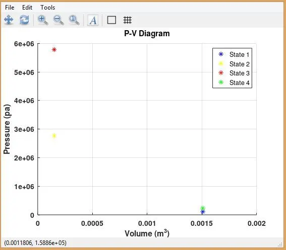
In order to determine a compression and expansion stroks of the state points for an operating cycle, need to trace a volume of compression and expansion curves. For that by using a function to determine the isentropic compression(v_compression) and isentropic expansion (v_expansion).By determining the volume trace, the compression after the initial states and expansion after the heat addition states are been plotted.

TO DETERMINE VOLUME TRACE:

%Creating a function to determine volume trace

function [v]=piston_kinematics(bore,stroke,con_rod,cr,start_crank,end_crank)

a=stroke/2;  %crank pin radius in (m)
R=con_rod/a;  %ratio of con_rod to crank pin radius
theta=linspace(start_crank,end_crank,100); %start_crank and end_crank anlgles
v_s=pi/4*bore^2*stroke %swept volume in (m^3)
v_c=v_s/(cr-1)         %clearence volume in (m^3)
v=v_s+v_c              %volume 

%In order to determine volume trace by using a relation,
%v/v_c=1+{(1/2)*(cr-1)}*{R+1-cosd(theta)}-{(R^2-sind(theta).^2).^0.5}
%It's can be segmented in 3 segments,

seg1=0.5*(cr-1); 
seg2=R+1-cosd(theta);
seg3=(R^2-sind(theta).^2).^0.5; %  .(dot)operator is used for element operation
% Volume trace are calculated as,
v=(1+seg1*(seg2-seg3)).*v_c; %combining the segments and multiplied with v_c

end

By calling the above function is used to determine the volume trace in compression and expansion stroks.By calling a function using the expression as,

In the above expression the inputs are defined by passing the values in the expression will results in determining the compression and expansion stokes.With that from initial state to heat addition stroke are plotted as isentropic compression. Also from after heat additon to heat rejection state are plotted as isentropic expansion.

PROGRAM FOR OTTO CYCLE USING MATLAB:

%Air standared cycle:
%There are 4 states 
clear all
close all
clc
% Consider Inputs
p1=110185; %initial pressure in (pascal)
t1=400; %initial temperature in (kelvin)
t3=2100; %peak temperature in (kelvin)
cr=10; %compression ratio
gamma=1.4; %specific heat ratio(cp/cv)

%Engine geometric parameters:
bore=0.12; %bore diameter in(m)
stroke=0.12; %stroke lengt in(m)
con_rod=0.20; %connecting rod length in (m)

%State variable 1:
%To find volume(V1) by swept volume and clearence volume

v_s=pi/4*bore^2*stroke; %swept volume in(m^3)
v_c=v_s/(cr-1); %clearence volume in(m^3)

v1=v_s+v_c; %volume 1 calculated

%State variable 2;

v2=v_c; %Pistion is at top dead center(TDC)so, v2 equals clearence volume

%To find pressure using relation,
%p1v1^gamma=p2v2^gamm  | p2=p1*(v1/v2)^gamma
%(v1/v2)=cr

p2=p1*(cr)^gamma; %pressure 2 calculated 

%To find temperature t2 by using ideal gas relation,
% p1v1/t1= p2v2/t2  | t2=p2*v2*t1/p1*v1

t2=p2*v2*t1/(p1*v1); %temperature t2 calculated
%By calling a function to determine v_compression & p_compression
%Piston is at compression state, start_crank_angle 180 and end crank angle 0

v_compression=piston_kinematics(bore,stroke,con_rod,cr,180,0); 

%To find out p_compression by using relation
% p_compression*v_compression^gamma=c |  p_compression=c./v_compression

c=p1*v1^gamma % To calculate constant (c)

p_compression=c./v_compression.^gamma;

%State Variable 3:

v3=v2; % at constant volume volumes v3=v2

%To find peak pressure p3 by using relation
%p2v2/t2=p3v3/t3  | p3=p2*(t3/t2)

p3=p2*(t3/t2); %pressure (p3) calculated
%By calling a function to determine v_expansion & p_expansion
%Piston is at expansion state,start_crank_angle 0 and end crank angle 180

v_expansion=piston_kinematics(bore,stroke,con_rod,cr,0,180);
%To find out p_expansion by using relation
% p_expansion*v_expansion^gamma=c |  p_expansion=c./v_expansion
%To calculate constant for the state point 3,
c=p3*v3^gamma %constant (c) calculated

p_expansion=c./v_expansion.^gamma

%State variable 4:

v4=v1  % at constant volume volumes v3=v2

%To find pressure(p4) by using relation
% p3v3^gamma=p4v4^gamma  | p4=p3*(v3/v4)^gamma

p4=p3*(v3/v4)^gamma % pressure(p4) calculated

%To find temperature t4 by using ideal gas relation,
% p3v3/t3= p4v4/t4  | t4=p4*v4*t3/p3*v3

t4=p4*v4*t3/p3*v3; %temperature t4 is calculated
% Plotting

figure(1)  %to get separate window plot
hold on    %retains the current plot and certain axes properties
plot(v1,p1,'*','color','b')       %state 1 values plotted
plot(v_compression,p_compression) %compression state are plotted 
plot(v2,p2,'*','color','y')       %state2 values plotted
plot([v2 v3],[p2 p3])             %to plot state 2 & state 3
plot(v3,p3,'*','color','r')       %state 3 values plotted
plot(v_expansion,p_expansion)     %expansion state plotted
plot(v4,p4,'*','color','g')       %state 4 values plotted
plot([v4 v1],[p4 p1])             %state 4 & state 1 plotted
grid on           
title('PV Diagram');              %add title in plot
xlabel('Volume (m^3)');           %labelling x-axis
ylabel('Pressure (pa)');           %labelling y-axis
set(gca,'fontweight','bold','fontsize',14) %current axis properties to change
legend('State 1','Isentropic Compression','State 2','Constant volume heat addition','State 3','Isentropic Expansion','State 4','Constant volume heat rejection')

%To find thermal efficiency

Efficiency=(1-1/cr^(gamma-1))*100 %calculated efficiency of an engine

PLOTTING OF AN P-V DIAGRAM:

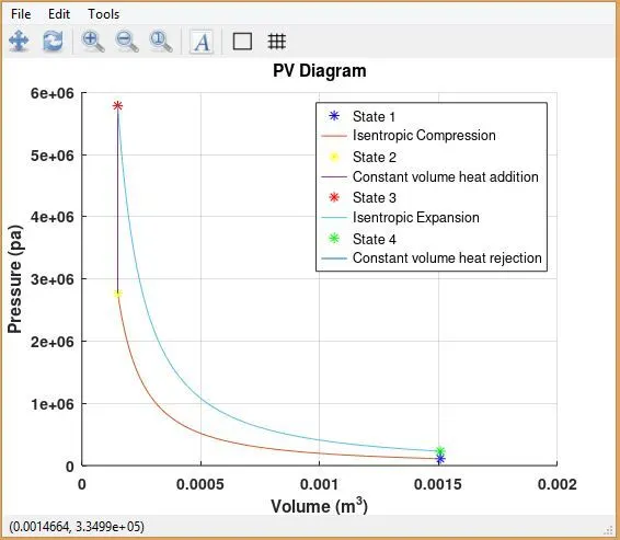
• The PV diagram clearly represents that when the piston performs work on the air-fuel mixture, the volume of the gas decreases (compresses) and pressure increases. Similarly, after combustion, the released heat by the mixture performs work on the piston due to that it expands (expansion process)..
• From the initial state 1 to state 2 the compression stroke is not linear it is formed as a curve as plotted.
• After the heat addition process the expansion stroke takes place in the curve as plotted.

CODING EXPLANATION:

• Assigning an inputs to the initial temperature, pressure, peak pressure,compression ratio,specific heat ratio.
• Assigning an inputs to crank pin radius,connecting rod length,bore, stroke length.
• Calculating the state variables by relations and ideal gas equations.(p1,v1,t1),(p2,v2,t2),(p3,v3,t3),(p4,v4,t4).
• To find the initial volume by using the engine geometric parameters.
• Swept volume and Clearence volume are calculated to determine volume(v1) at initial state
• The realtion p*v^gamma=constant is used to determine the pressure at required state points
• The ideal gas equation PV=MRT is used to detremine the required tempetatures at state points
• After the initial state the piston moves from BDC to TDC for compression stroke where v_compression and p_compression are derived by calling a function.
• A function is defined to get the output of values which are passing from the inputs.
• In the function the equations are been segmented into tree segments as, seg1,seg2,and seg3.
• Piston is at compression state, start_crank_angle 180 and end_crank angle 0
• To detremine the volume trace the segments are derivred and with that clearence volume are multiplied.
• By the functions v_compression and p_compression are determined
• Then, after the heat addition process the piston moves from TDC to BDC for expansion stroke.
• Piston is at expansion stroke, start_crank_angle 0 and end_crank angle 180
• By the functions and relations v_expansion and p_expansions are determined
• Determining the state points,comptession and expansion strokes plotting is done
• Finally the thermal efficiency of an engine is calculated by using the realtion (1-1/cr^(gamma-1))*100

ERRORS FACED WHILE PROGRAMMING:

• dot (.) operator is not used in element opeartion during expansion stroke

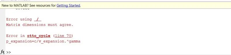
• Unrecgonized variable founded

STEPS TO OVERCOME ERRORS:

• dot(.) operator is used in element wise operations
• Multiplication is used in respected variable

RESULTS:

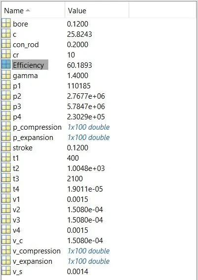
The state points pressure, volume and temperature are founded. Isentropic process are also determined.

THERMAL EFFICIENCY:

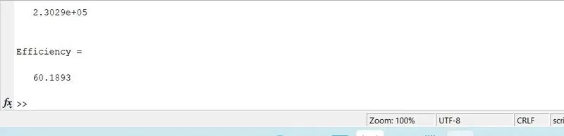
• Thermal efficiency of an engine are determined in matlab by using codes and it is found to be 60.189%

• The thermal efficiency of the Otto cycle depend on the compression.

• A higher compression ratio decreases fuel consumption at the same temperature, allowing longer cycles of expansion.
• There will be more electric power and a lower exhaust gas temperature. Reducing track temperature decreases ambient energy pollution

CONCLUSION:

• By using matlab, program has been done for an otto cycle
• PV Diagram are plotted
• Thermal efficiency of an engine are founded.