Project

CURVE FITTING USING MATLAB

VVenkatesh K30 Jan 2022

MATLAB

AIM:

TO write a code to fit a linear and Cubic polynomial for the given data’s and to write a code to show splitwise method.

OBJECTIVE:

1. Plot the linear and cubic fit curves along with the raw data points.

2. Explain the parameters used to measure the fitness characteristics

3. Validate fitness characteristics using Matlab tool

INTRODUCION:

CURVE FITTING:

The curve fitting is a process of constructing a curve and to find the parameters of a mathematical model that describes a set of data in a way that minimizes the difference between the model and the data. The most common approach is the "linear least squares" method, also called "polynomial least squares", a well-known mathematical procedure for finding the coefficients of polynomial equations that are a "best fit" to a set of X,Y data. A polynomial equation expresses the dependent variable Y as a polynomial in the independent variable X.

POLYFIT:

Polyfit is a Matlab function that computes a least squares polynomial for a given set of data.It can be written as polyfit(x,y,n) where n is the order of polynomial. Polyfit generates the coefficients of the polynomial, which can be used to model a curve to fit the data.

POLYVAL:

Polyval evaluates a polynomial for a given set of x values. So, Polyval generates a curve to fit the data based on the coefficients found using polyfit.It can be writtern as, polyval(co-efficients,x)

PARAMETERS USED TO MEASURE THE GOODNESS OF FIT:

A goodness-of-fit is a statistical analysis that determine whether a set of observed values match those expected under the applicable model. There are four methods to evaluate the goodness of fit,

(1) The sum of squares due to error (SSE)

(2) R-square

(3) Adjusted R-square

(4) Root mean squared error (RMSE)

(1) The sum of squares due to error (SSE):

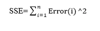
This statistic measures the total deviation of the response values from the fit to the response values. It is also called the summed square of residuals and is usually labeled as SSE. A value closer to 0 indicates that the model has a smaller random error component, and that the fit will be more useful for prediction.

(2) R-square:

This statistic measures how successful the fit is in explaining the variation of the data. R-square is the square of the correlation between the response values and the predicted response values. It is also called the square of the multiple correlation coefficient and the coefficient of multiple determination. R-square is defined as the ratio of the sum of squares of the regression (SSR) and the total sum of squares (SST).

R²=SSR/SST

Where,

SSR=Sum of Squared Regression, The sum of squared differences between predicted data points and the mean of the response variable.

To evaluate SSR as,

SST=Total Sum of Suqare

SST=SSR+SSE

R-square can take on any value between 0 and 1, with a value closer to 1 indicating that a greater proportion of variance is accounted for by the model. Value close to 1 indicates better fit.

(3) Adjusted R-square:

This statistic uses the R-square statistic and adjusts it based on the residual degrees of freedom.

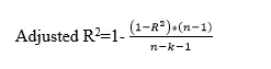
Where k, indicates the number of independent pieces of information involving

n, data points that are required to calculate the sum of squares.

The adjusted R-square statistic is generally the best indicator of the fit quality when you compare two models that are nested. The adjusted R-square statistic can take on any value less than or equal to 1, with a value closer to 1 indicating a better fit.

(4) Root mean squared error (RMSE):

This statistic is also known as the fit standard error and the standard error of the regression. It is an estimate of the standard deviation of the random component in the data, and is defined as,

RMSE=sqrt (SSE/n)

CASES INVOLVED IN CODING:

CASE (1): CODE TO FIT A LINEAR POLYNOMIAL FOR CP_ DATA

CASE (2): CODE TO FIT A CUBIC POLYNOMIAL FOR CP_ DATA

CASE (3): SPLIT WISE METHOD

STEPS IN CODING:

STEP 1: Load a data and Define the respective data's as temperature and specific_heat

STEP 2: Detremine the co-efficients using polyfit command

STEP 3: Assigning the co-efficients in polyval command to determine predicted data

STEP 4: Comparing the original data set with predicted data set

STEP 5: In order to compare original data set with predicted data plotting is done

STEP 6: Evaluate the goodness of fit analytically using four statstical methods

STEP 7: Validating the goodness of fit using cf tool in Matlab

CODING:

CASE (1): CODE TO FIT A LINEAR POLYNOMIAL FOR CP_ DATA

%To write a code to fit linear polynomial 
clear all 
close all
clc
%Loading a data
cp_data=load('data'); %used to prepare a data's
temperature=cp_data(:,1); %select the first column as temperature
specific_heat=cp_data(:,2); %select the second column as temperature

%Curve fitting for linear polynomial (n=1)

co_effi=polyfit(temperature,specific_heat,1); %finding the co-efficients

pred_specific_heat=polyval(co_effi,temperature); %determine the predicted data's

%comparing original data with predicted data's for linear polynomial

figure(1) %To create seperate window figure
plot(temperature,specific_heat,'r','linewidth',2); %plotting original data
hold on %hold the current polt and execute the next plot
plot(temperature,pred_specific_heat,'b','linewidth',2); %plotting the predicted data
grid on
xlabel('Temperature [k]'); %for x labelling
ylabel('Specific Heat [KJ/K-mol K]'); %for y labelling
axis([0 3500 900 1400]); %setting x & y axis
title('Specific heat vs Temperature');
set(gca,'fontsize',14);
legend('Original data set','Predicted data set','location','northwest');

%Measure goodness of a fit 
M=mean(specific_heat); %calculating mean value of specific_heat
Error1=(pred_specific_heat-specific_heat).^2 ;%Determining the error
%Sum of Squared Error-(SSE)
SSE=sum(Error1);
%To find Sum of Squared Regression-(SSR)
ssr=(pred_specific_heat-M)^.2;
SSR=sum(ssr);
%To find Total Sum of Square-(SST)
SST=SSR+SSE;
%Calculating R_square
R_sqr=(SSR/SST);

%To measure Adj R_square
n=3200; %Number of data points
k=1;  % Represents the independant variable

% To Measure Adj r_square

Adj_R_square=1-(((1-R_sqr)*(n-1))/(n-k-1));

%To measure Root Mean Squared Error

RMSE=sqrt(SSE/n);

PLOTTING:

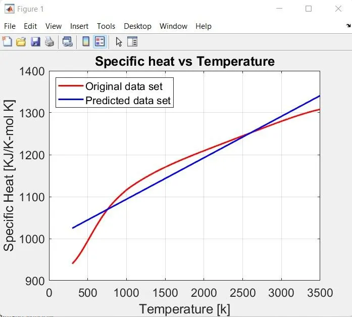
Figure(1) describes the plotting and comparision of original data set with predicted data set. For the polynomial orderof n=1 there are so many variations are obsorved in the plot and curve also doesn't fitts properly

VALIDATING GOODNESS OF FIT USING CF-TOOL:

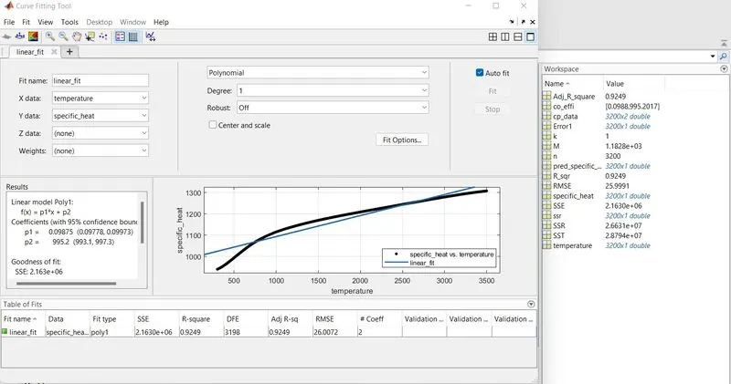
By validating the linear fit with cf tool and analyticallyit is obsorved as the value of R_square is 0.9249 that is 92.49%.

it is not to be considered as a perfect fit.

CASE (2): CODE TO FIT A CUBIC POLYNOMIAL FOR CP_ DATA:

%To write a code to fit cubic polynomial 
clear all 
close all
clc
%Loading a data
cp_data=load('data'); %used to prepare a data's
temperature=cp_data(:,1); %select the first column as temperature
specific_heat=cp_data(:,2); %select the second column as temperature

%Curve fitting for cubic polynomial(n=3)

co_effi=polyfit(temperature,specific_heat,3); %finding the co-efficients

pred_specific_heat=polyval(co_effi,temperature); %determine the predicted data's

%comparing original data with predicted data's

figure(2) %To create seperate window figure
plot(temperature,specific_heat,'r','linewidth',2);%plotting original data
hold on
plot(temperature,pred_specific_heat,'b','linewidth',2);%plotting the predicted data
grid on
xlabel('Temperature [k]');%for x labelling
ylabel('Specific Heat [KJ/K-mol K]'); %for y labelling
axis([0 3500 900 1400]);%setting x & y axis
title('Specific heat vs Temperature');
set(gca,'fontsize',14);
legend('Original data set','Predicted data set','location','northwest');

%Measure goodness of a fit 
M=mean(specific_heat); %calculating mean value of specific_heat
Error2=(pred_specific_heat-specific_heat).^2 ;%Determining the error
%Sum of Squared Error-(SSE)
SSE=sum(Error2);
%To find Sum of Squared Regression-(SSR)
ssr=(pred_specific_heat-M).^2;
SSR=sum(ssr);
%To find Total Sum of Square-(SST)
SST=SSR+SSE;
%Calculating R_square
R_sqr=(SSR/SST);

%To measure Adj R_square
n=3200; %Number of data points
k=1;  % Represents the independant variable

% To evaluate Adj r_square

Adj_R_square=1-(((1-R_sqr)*(n-1))/(n-k-1));

%To measure Root Mean Squared Error

RMSE=sqrt(SSE/n);

PLOTTING:

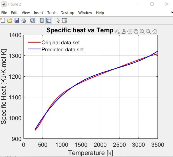
Figure(2) describes the plotting and comparision of original data set with predicted data set. For the polynomial orderof n=3 tit is obsorved that in the plot and curve fitts properly and hence it is having fewer variations.

VALIDATING GOODNESS OF FIT USING CF-TOOL:

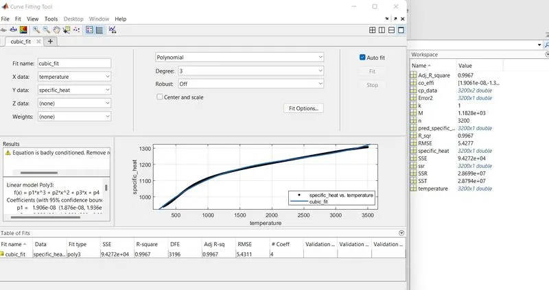
By validating the cubic fit with cf tool and analyticallyit is obsorved as the value of R_square is 0.9967 that is 99.67%. It is considered as a best fit. Also in the cubic fit while assigning the polynomial of n=3, it gives an error called as Equation is badly conditioned. So, for that the data's are segmented/splitted into number of categories to determine the best fit and centering and scaling is used to fit the curve perfectly.Spli-wise method is used to split the temperature and specific heat ranges into sub-groups.

BASED ON THE RESEARCH:

1. How to make a curve fit perfectly?

In order to get the curve fit perfectly,the degree of polynomial are incresed using cf tool, the polynomial order of 8th will give the perfect fit.

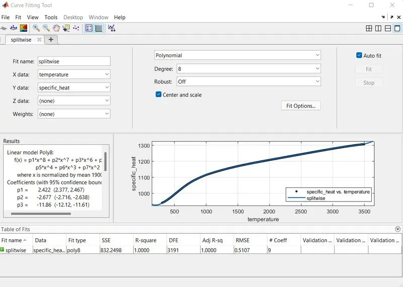
By increasing the order of polynomial to 8 the curve fits perfectly and the value of R_square and Adjusted R_Square are measured as 1 thatis 100% the curve fitt with the original data's. Without error estimations.

2. How to get the best fit?

Best fit simply means that the differences between the actual measured specific heat values and the specific heat values predicted by the model equation are minimized. It does not mean a "perfect" fit; in most cases, a least-squares best fit does not go through all the points in the data set. A least-squares fit must conform to the selected model. The data are not being modified in any way, it is the model that is being adjusted to fit the data.

3.What could be done to improve the cubic fit?

To improve the cubic fit, the data are splitted into number of ranges and by centering and scalling functions the cubic fit is done perfectly.

CODING:

CASE (3): SPLIT WISE METHOD:

%Splitwise method for curve fit
clear all
close all
clc
%Loading a data

cp_data=load('data'); %used to prepare a data's
temperature=cp_data(:,1); %select the first column as temperature
specific_heat=cp_data(:,2); %select the second column as temperature

%curve fitting
co_effi=polyfit(temperature,specific_heat,3); %finding the co-efficients

pred_specific_heat=polyval(co_effi,temperature); %determine the predicted data's

%splitting the data's into 4 sub-groups
%splitting temperature data from cp_data

t1=temperature(1:800);     %Splitting temperature range as t1
t2=temperature(801:1600);  %Splitting temperature range as t2
t3=temperature(1601:2400); %Splitting temperature range as t3
t4=temperature(2401:3200); %Splitting temperature range as t4
c_T=[t1;t2;t3;t4];         %Cumulative temperature

%splitting specific_heat data's
s_h1=specific_heat(1:800);     %Splitting specific_heat range s_h1
s_h2=specific_heat(801:1600);  %Splitting specific_heat range s_h2
s_h3=specific_heat(1601:2400); %Splitting specific_heat range s_h3
s_h4=specific_heat(2401:3200); %Splitting specific_heat range s_h4

c_s_h=[s_h1;s_h2;s_h3;s_h4];   %Cumulative specific heat

%curve fitting for splitwise method using centering and scalling
%curve fitting for t1,s_h1

[co_effi1,~,mu]=polyfit(t1,s_h1,3);    
pred_s_h_1=polyval(co_effi1,t1,[],mu);  %predicted split range 1:800
%curve fitting for t2,s_h2

[co_effi2,~,mu]=polyfit(t2,s_h2,3);
pred_s_h_2=polyval(co_effi2,t2,[],mu);  %predicted split range 800:1600

%curve fitting for t3,s_h3

[co_effi3,~,mu]=polyfit(t3,s_h3,3);
pred_s_h_3=polyval(co_effi3,t3,[],mu);  %predicted split range 160:2400

%curve fitting for t4,s_h4

[co_effi4,~,mu]=polyfit(t4,s_h4,3);
pred_s_h_4=polyval(co_effi4,t4,[],mu);  %predicted split range 2400:3200

c_pred_s_h=[pred_s_h_1;pred_s_h_2;pred_s_h_3;pred_s_h_4]; %Cumulative predictedspecific heat

%comparing original data with predicted data's
figure(3)
plot(temperature,specific_heat,'g','linewidth',4); %plot original data set
hold on
plot(t1,pred_s_h_1,'b','linewidth',2);  %plot predicted range 1
hold on
plot(t2,pred_s_h_2,'r','linewidth',2);  %plot predicted range 2
hold on
plot(t3,pred_s_h_3,'y','linewidth',2);  %plot predicted range 3
hold on
plot(t4,pred_s_h_4,'c','linewidth',2);  %plot predicted range 4
grid on
xlabel('Temperature [k]'); %for x labelling
ylabel('Specific Heat [KJ/K-mol K]');%for y labelling
axis([0 3500 900 1400]);
title('Specific heat vs Temperature');
set(gca,'fontsize',14);
legend('Original data set','Split range 1','Split range 2','Split range 3','Split range 4','location','northwest')

PLOTTING:

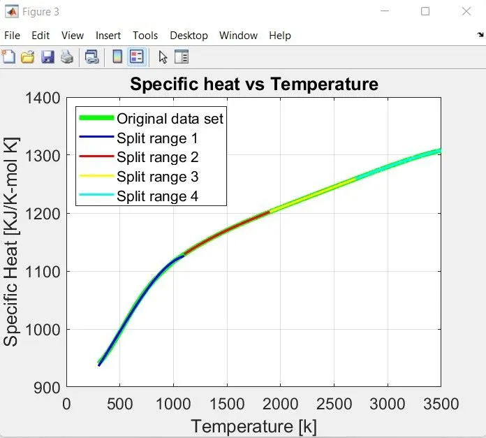
Figure(3) describes the plotting and comparision of original data set with predicted data se by splitwise method. For the polynomial orderof n=3 tit is obsorved that in the plot and curve fitts properly.

VALIDATING SPLITWISE METHOD USING CF-TOOL:

CENTERING AND SCALLING:

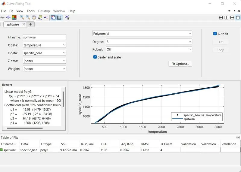
By splitwise method the curves are perfectly fitted and using centering and scalling functions to get the smotter curves.It is obsorved thaat 99.67% the curve fits perfectly by the splitwise method.

CODING EXPLANATION:

Loading the data using load command and defining the temperature and specific heat of the data's respectively.
Determining the co-efficients of the data using polyfit command.
In the polyfit command assign the inputs x and y.
Also, assign the polynomial such as linear(n=1) and cubic polynomials(n=3)
Polyfit command returns co-efficients, that will be used to predict the data for curve fitting.
With the predicted dat's plot with original data'a to relate
Plotting is done for original data and predicted specific heat data's
Labelling the plots of x and y axis as,temperature(k) and specific heat (kj/k mol k)respectively.
Assigning the legends to describe the plotted original data set and predicted data set.
Then, after the grapical representation the goodness of the fit are measured using four important parameters
To evaluate the goodness need to detremine the SSE, R_Square,Adjusted R_Square and RMSE.
After evaluation of goodnedss fit validation has been done using Matlab software cf tool

ERROS FACED WHILE CODING:

In the element wise operation the dot (.) operation was not done in evaluating the goodness of fit

STEPS TO OVERCOME THOSE ERRORS:

For Element wise operation dot(.) was assignied correctly.

CONCLUSION:

In order to make a fit perfectly the order of polynomial is increased.
The splitting the data's and evaluating it to make the curve more perfectly.
A coding has been done to fit linear and cubic polynomials
Coding has been done using splitwise method

REFERENCE:

CURVE FITTING USING MATLAB

Ship work like this
in your own course.

Talk to a career counsellor

Ship work like thisin your own course.

Talk to a career counsellor

Ship work like this
in your own course.