Week 7 - Simulation of a 1D Super-sonic nozzle flow simulation using Macormack Method

Objective:

To apply MacCormack's approach in MATLAB to solve the governing equations and simulate the isentropic flow via a quasi-1-dimensional subsonic nozzle by deriving both the conservation and non-conservation versions of the equations.

Statement:

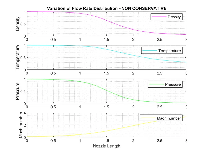
By comparing their solutions with the figures below, it is possible to ascertain the steady-state temperature distribution for the flow-field variables and study the differences between the two types of governing equations.

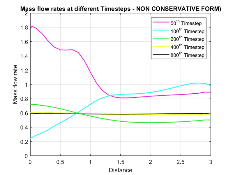
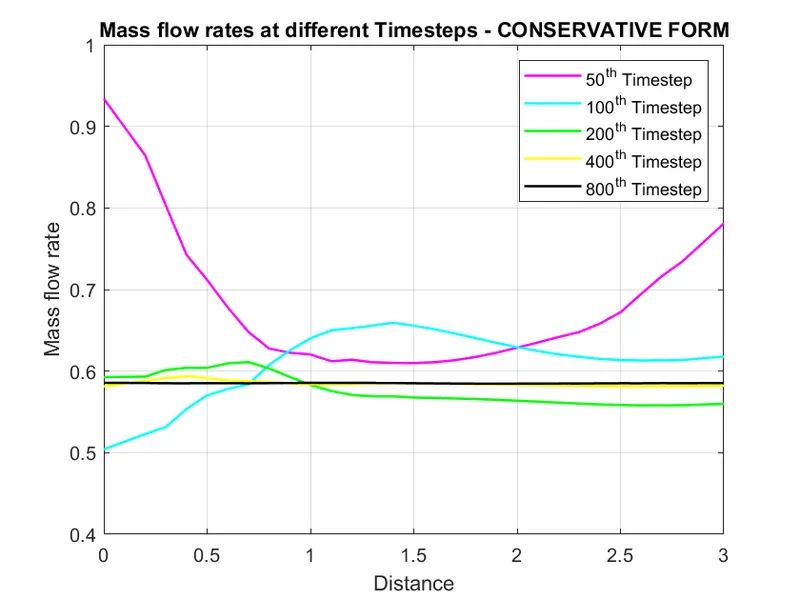
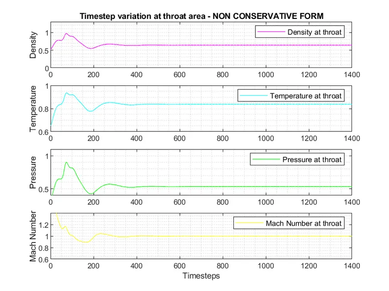
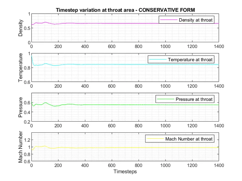
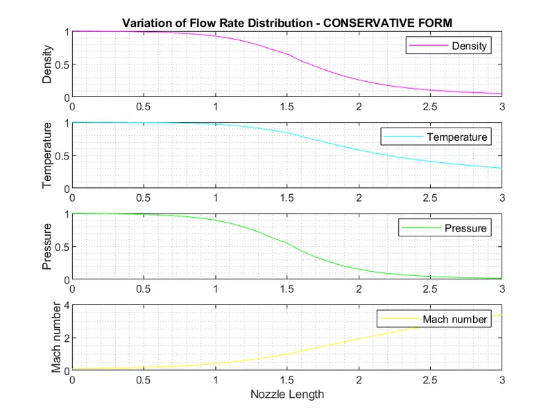
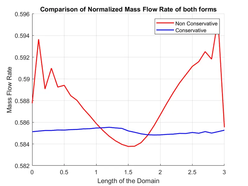
Inside the nozzle, there is a steady-state distribution of the primitive variable.The basic variable's temporal fluctuation. During the time-marching operation, the mass rate distribution within the nozzle changes at various time steps. Comparison of both kinds' normalised mass flow rate distributions.

Theory:

There is an analytical solution for this kind of issue, hence any numerical solution of isentropic flow via a quasi-1D subsonic-supersonic nozzle is absurd. However, rather than accurately expressing the approximate form of an analytical solution, we are attempting to demonstrate the expanded capacity of CFD in diverse streams. Here, we use conservative and nonconservative forms to accomplish the numerical answer.

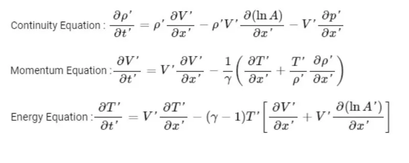
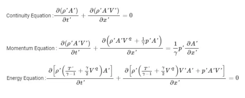
In order to employ Time Marching to solve the issue, governing equations are marched in terms of PDE for both forms. These forms simply represent in a numerical sense; all analytical techniques follow the same patterns.

Non-Conservative form:

Conservative form:

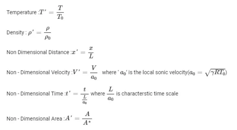
Non-Dimensional Quantities:

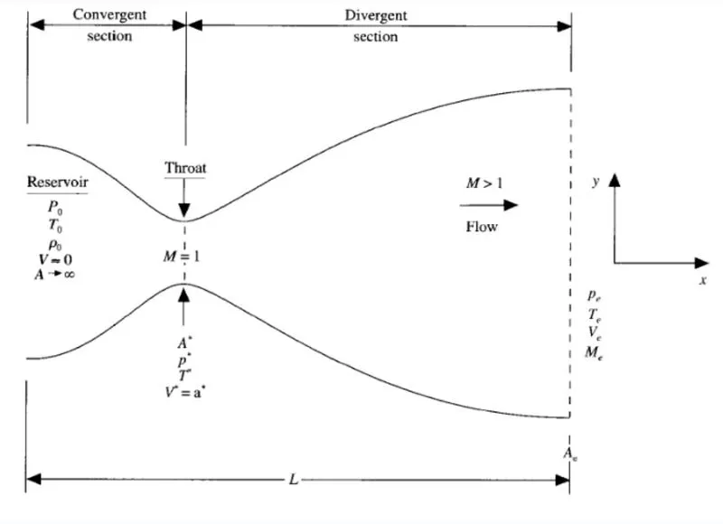
Nozzle diagram:

There are two types of convergent sections and divergent sections.

MacCormack method:

To discretize the numerical solution we use the technique called the MacCormack method. The MacCormack method is a variation of the two-step Lax-Wendroff Scheme but is much simpler in the application.

The application of the MacCormack method proceeds in two steps; a predictor step which is followed by a corrector step.

Predictor step: In the predictor step, a "provisional" value of u at time level n+1 (denoted by u_i^n+1) is estimated and obtained by replacing the spatial and temporal derivatives in the previous first-order equation using the Forward Difference Scheme. Delta t is used for Timestep.

Corrector step: In the corrector step, the predicted value u_i^n+1 is corrected according to the equation. Note that the corrector step uses the Backward Difference Scheme for spatial derivative. The time-step used in the corrector step is Delta t/2 in contrast to the Delta t used in the predictor step.

Main Program:

In order for the code to be modular, the program is split into three sections. They are

Main Program of Quasi 1D subsonic-supersonic nozzle

Two functions namely

Non Conservative form.
Conservative form.

clear all
close all
clc

%SOLVING QUASI 1D SUPERSONIC NOZZLE FLOW EQUATIONS
%Shriyash Tamhane
%INPUT PARAMETERS
%No. of grid points    
n = 31;             

gamma = 1.4;
x = linspace(0,3,n);
dx = x(2) - x(1);

%No. of time step
nt = 1400;

%Courant Number
C = 0.5;            


%FUNCTION FOR NON CONSERVATIVE FORM
tic;
[Mass_flow_rate_NC, Pressure_NC, Mach_number_NC, rho_NC, v_NC, T_NC, rho_throat_NC, v_throat_NC, T_throat_NC, Mass_flow_rate_throat_NC, Pressure_throat_NC, Mach_number_throat_NC] = Non_conservative_form(x, dx, n, gamma, nt, C);
Time_elapsed_NC = toc;
fprintf('Time Elasped for Non Conservative form: %0.4f', Time_elapsed_NC);
hold on

%PLOTTING 
%Timestep variation of properties at throat area in Non Conservative form
figure(2)

%Density
subplot(4,1,1)
plot(linspace(1,nt,nt),rho_throat_NC,'color','m')
ylabel('Density')
legend({'Density at throat'});
axis([0 1400 0 1.3]);
grid minor;
title('Timestep variation at throat area - NON CONSERVATIVE FORM')

%Temperature
subplot(4,1,2)
plot(linspace(1,nt,nt),T_throat_NC,'color','c')
ylabel('Temperature')
legend({'Temperature at throat'});
axis([0 1400 0.6 1]);
grid minor;

%Pressure
subplot(4,1,3)
plot(linspace(1,nt,nt),Pressure_throat_NC,'color','g')
ylabel('Pressure')
legend({'Pressure at throat'});
axis([0 1400 0.4 1.1]);
grid minor

%Mach Number
subplot(4,1,4)
plot(linspace(1,nt,nt),Mach_number_throat_NC,'color','y')
xlabel('Timesteps')
ylabel('Mach Number')
legend({'Mach Number at throat'});
axis([0 1400 0.6 1.4]);
grid minor;


%Steady state simulation for primitve values for Non Conservative form
figure(3);
%Density

subplot(4,1,1);
plot(x,rho_NC,'color','m')
ylabel('Density')
legend({'Density'});
axis([0 3 0 1])
grid minor;
title('Variation of Flow Rate Distribution - NON CONSERVATIVE')

%Temperature
subplot(4,1,2);
plot(x,T_NC,'color','c')
ylabel('Temperature')
legend({'Temperature'});
axis([0 3 0 1])
grid minor;

%Pressure
subplot(4,1,3);
plot(x,Pressure_NC,'color','g')
ylabel('Pressure')
legend({'Pressure'});
axis([0 3 0 1])
grid minor;

%Mach number
subplot(4,1,4);
plot(x,Mach_number_NC,'color','y')
xlabel('Nozzle Length')
ylabel('Mach number')
legend({'Mach number'});
axis([0 3 0 4])
grid minor;


%FUNCTION FOR CONSERVATIVE FORM
tic;
[Mass_flow_rate_C, Pressure_C, Mach_number_C, rho_C, v_C, T_C, rho_throat_C, v_throat_C, T_throat_C, Mass_flow_rate_throat_C, Pressure_throat_C, Mach_number_throat_C] = Conservative_form(x, dx, n, gamma, nt, C);
Time_elasped_C = toc;
fprintf('Time Elasped for Conservative form: %0.4f', Time_elasped_C);

%PLOTTING 
%Timestep variation of properties at throat area in Conservative form
figure(5)

%Density
subplot(4,1,1)
plot(rho_throat_C,'color','m')
ylabel('Density')
legend({'Density at throat'});
axis([0 1400 0 1]);
grid minor;
title('Timestep variation at throat area - CONSERVATIVE FORM')

%Temperature
subplot(4,1,2)
plot(T_throat_C,'color','c')
ylabel('Temperature')
legend({'Temperature at throat'});
axis([0 1400 0.6 1]);
grid minor;

%Pressure
subplot(4,1,3)
plot(Pressure_throat_C,'color','g')
ylabel('Pressure')
legend({'Pressure at throat'});
axis([0 1400 0.2 0.8]);
grid minor

%Mach Number
subplot(4,1,4)
plot(Mach_number_throat_C,'color','y')
xlabel('Timesteps')
ylabel('Mach Number')
legend({'Mach Number at throat'});
axis([0 1400 0.6 1.4]);
grid minor;


%Steady state simulation for primitve values for Non Conservative form
figure(6);

%Density 
subplot(4,1,1);
plot(x,rho_C,'color','m')
ylabel('Density')
legend({'Density'});
axis([0 3 0 1])
grid minor;
title('Variation of Flow Rate Distribution - CONSERVATIVE FORM')

%Temperature 
subplot(4,1,2);
plot(x,T_C,'color','c')
ylabel('Temperature')
legend({'Temperature'});
axis([0 3 0 1])
grid minor;

%Pressure
subplot(4,1,3);
plot(x,Pressure_C,'color','g')
ylabel('Pressure')
legend({'Pressure'});
axis([0 3 0 1])
grid minor;

%Mach number
subplot(4,1,4);
plot(x,Mach_number_C,'color','y')
xlabel('Nozzle Length')
ylabel('Mach number')
legend({'Mach number'});
axis([0 3 0 4])
grid minor;


%COMPARISON PLOT of Normalized Mass Flow Rate of both forms
figure(7)
hold on
plot(x,Mass_flow_rate_NC,'r','linewidth',1.5)
hold on;
plot(x,Mass_flow_rate_C,'b','linewidth',1.5)
hold on;
grid on

legend('Non Conservative','Conservative');
xlabel('Length of the Domain')
ylabel('Mass Flow Rate')
title('Comparison of Normalized Mass Flow Rate of both forms')

Explanation:

Clear all, close all, and clc are used at the beginning of code to start over without changing any of the values from before.
The variables x, dx, n, gamma, nt, and C all have input parameters that are set.
Non-conservative and conservative forms are made as separate functions with the inputs needed, which are explained below.

The tic-toc command is used to figure out how much time has passed between two events.

For the following problems, plans are made:

1) Both forms' throats have different timesteps

2)Variation of both forms of flow rate distribution

3)Compare the two types of normalised mass flow rate

Each plot is made up of four subplots: density, temperature, pressure, and the Mach number at the throat, as well as the converging/diverging section.

NON-CONSERVATIVE FORM:

%Function for Non-Conservative form

function [Mass_flow_rate_NC, Pressure_NC, Mach_number_NC, rho_NC, v_NC, T_NC, rho_throat_NC, v_throat_NC, T_throat_NC, Mass_flow_rate_throat_NC, Pressure_throat_NC, Mach_number_throat_NC] = Non_conservative_form(x, dx, n, gamma, nt, C)

%Intial boundary conditions
rho_NC = 1 - 0.3146*x;
T_NC = 1 - 0.2341*x;
v_NC = (0.1 + 1.09*x).*T_NC.^0.5;

%Area & Throat profiles
a = 1 + 2.2*(x - 1.5).^2;
throat = find(a==1);


%Outer Time Loop
for k = 1:nt
    
    %Time-step control
    dt = min(C.*dx./(sqrt(T_NC) + v_NC));
    
    %Saving a copy of Old Values
    rho_old = rho_NC;
    T_old = T_NC;
    v_old = v_NC;
    

    %Predictor Method
    for j = 2:n-1
        
        %Simplifying the Equation's spatial terms
        dv_dx = (v_NC(j + 1) - v_NC(j))/dx;
        drho_dx = (rho_NC(j + 1) - rho_NC(j))/dx;
        dT_dx = (T_NC(j + 1) - T_NC(j))/dx;
        dlog_a_dx = (log(a(j + 1)) - log(a(j)))/dx;
        
        %Continuity Equation
        drho_dt_P(j) = -rho_NC(j)*dv_dx - rho_NC(j)*v_NC(j)*dlog_a_dx - v_NC(j)*drho_dx;
        
        %Momentum Equation
        dv_dt_P(j) = -v_NC(j)*dv_dx - (1/gamma)*(dT_dx + (T_NC(j)*drho_dx/rho_NC(j)));
        
        %Energy Equation
        dT_dt_P(j) = -v_NC(j)*dT_dx - (gamma - 1)*T_NC(j)*(dv_dx + v_NC(j)*dlog_a_dx);
        
        
        %Solution Update
        rho_NC(j) = rho_NC(j) + drho_dt_P(j)*dt;
        v_NC(j) = v_NC(j) + dv_dt_P(j)*dt;
        T_NC(j) = T_NC(j) + dT_dt_P(j)*dt;
        
    end
    
    
    %Corrector Method
    for j = 2:n-1
        
        %Simplifying the Equation's spatial terms
        dv_dx = (v_NC(j) - v_NC(j - 1))/dx;
        drho_dx = (rho_NC(j) - rho_NC(j - 1))/dx;
        dT_dx = (T_NC(j) - T_NC(j - 1))/dx;
        dlog_a_dx = (log(a(j)) - log(a(j - 1)))/dx;
        
        %Continuity Equation
        drho_dt_C(j) = - rho_NC(j)*dv_dx - rho_NC(j)*v_NC(j)*dlog_a_dx - v_NC(j)*drho_dx;
        
        %Momentum Equation
        dv_dt_C(j) = - v_NC(j)*dv_dx - (1/gamma)*(dT_dx + (T_NC(j)*drho_dx/rho_NC(j)));
        
        %Energy Equation
        dT_dt_C(j) = - v_NC(j)*dT_dx - (gamma - 1)*T_NC(j)*(dv_dx + v_NC(j)*dlog_a_dx);
       
    end
    
    %Compute Average Time derivative
    drho_dt = 0.5.*(drho_dt_P + drho_dt_C);
    dv_dt = 0.5.*(dv_dt_P + dv_dt_C);
    dT_dt = 0.5.*(dT_dt_P + dT_dt_C);
    
    %Final Solution Update
    for i = 2:n-1
        rho_NC(i) = rho_old(i) + drho_dt(i)*dt;
        v_NC(i) = v_old(i) + dv_dt(i)*dt;
        T_NC(i) = T_old(i) + dT_dt(i)*dt;
        
    end
    
    %Applying Boundary Conditions
    %At Inlet
    rho_NC(1) = 1;
    v_NC(1) = 2*v_NC(2) - v_NC(3);
    T_NC(1) = 1;
    
    %At Outlet
    rho_NC(n) = 2*rho_NC(n-1) - rho_NC(n - 2);
    v_NC(n) = 2*v_NC(n - 1) - v_NC(n - 2);
    T_NC(n) = 2*T_NC(n - 1) - T_NC(n - 2);
    
    
    %Defining Mass flow rate, Pressure and Mach number
    Mass_flow_rate_NC = rho_NC.*a.*v_NC;
    Pressure_NC = rho_NC.*T_NC;
    Mach_number_NC = (v_NC./sqrt(T_NC));
    
    %Calculating Variables at throat section
    rho_throat_NC(k) = rho_NC(throat);
    T_throat_NC(k) = T_NC(throat);
    v_throat_NC(k) = v_NC(throat);
    Mass_flow_rate_throat_NC(k) = Mass_flow_rate_NC(throat);
    Pressure_throat_NC(k) = Pressure_NC(throat);
    Mach_number_throat_NC(k) = Mach_number_NC(throat);
    
    
    %PLOTTING
    %Comparison of non-dimensional Mass flow rates at different time steps
    figure(1);
    if k == 50
       plot(x, Mass_flow_rate_NC, 'm', 'linewidth', 1.25);
       hold on
    elseif k == 100
       plot(x, Mass_flow_rate_NC, 'c', 'linewidth', 1.25);
       hold on
    elseif k == 200
       plot(x, Mass_flow_rate_NC, 'g', 'linewidth', 1.25);
       hold on
    elseif k == 400
       plot(x, Mass_flow_rate_NC, 'y', 'linewidth', 1.25);
       hold on
    elseif k == 800
       plot(x, Mass_flow_rate_NC, 'k', 'linewidth', 1.25);
       hold on
    end
    
    %Labelling
    title('Mass flow rates at different Timesteps - NON CONSERVATIVE FORM)')
    xlabel('Distance')
    ylabel('Mass flow rate')
    legend({'50^t^h Timestep','100^t^h Timestep','200^t^h Timestep','400^t^h Timestep','800^t^h Timestep'})
    axis([0 3 0 2])
    grid on
    
end

end

Explanation:

The function's task is to use the known equations to figure out the values of Mass flow rate, Pressure, Mach number, Density, velocity, Temperature, Density at throat, velocity at throat, Temperature at throat, Mass flow rate at throat, Pressure at throat, and Mach number at throat for each grid point.

For this, initial boundary conditions for density, temperature, and speed, as well as profiles for figuring out area and throat, are set.
Now, the Outer Time loop is calculated for the for loop in order to figure out all the grid points for the different formulas inside the loop.
With the MacCarmack method, you can find the numerical solution to governing equations like the Continuity, Momentum, and Energy Equations.
The technique calls for two ways to solve problems: the Predictor method and the Corrector method.
Inside the for loop, the Predictor and Corrector methods are assigned separately so that values can be calculated.
In the next step, the values that have been calculated are averaged, and old values are added to the solution.
Boundary conditions are set up in the for loop and then used to figure out the Mass Flow Rate, Mach Number, Pressure, and throat section values.
Distance(x) and Mass Flow Rate for different Timesteps are finally plotted.
Program is ended.

CONSERVATIVE FORM:

%Function for Conservative form

function [Mass_flow_rate_C, Pressure_C, Mach_number_C,  rho_C, v_C, T_C, rho_throat_C, v_throat_C, T_throat_C, Mass_flow_rate_throat_C, Pressure_throat_C, Mach_number_throat_C] = Conservative_form(x, dx, n, gamma, nt, C)

%Determining Initial profile of Density and Temperature
for i = 1:n
    
    if (x(i) >= 0 && x(i) <= 0.5)
        rho_C(i) = 1;
        T_C(i) = 1;
    elseif (x(i) >= 0.5 && x(i) <= 1.5)
        rho_C(i) = 1 - 0.366*(x(i) - 0.5);
        T_C(i) = 1 - 0.167*(x(i) - 0.5);
    elseif (x(i) >= 1.5 && x(i) <= 3)
        rho_C(i) = 0.634 - 0.3879*(x(i) - 1.5);
        T_C(i) = 0.833 - 0.3507*(x(i) - 1.5);
    end
    
end

%Area & Throat profiles
a = 1 + 2.2*(x - 1.5).^2;
throat = find(a==1);

%Initial profile fot Velocity and Pressure
v_C = 0.59./(rho_C.*a);
Pressure_C = rho_C.*T_C;

%Calculate the Initial Solution Vectors(U)
U1 = rho_C.*a;
U2 = rho_C.*a.*v_C;
U3 = rho_C.*a.*(T_C./(gamma - 1)) + ((gamma/2).*v_C.^2);


%Outer Time Loop
for k =1:nt
    
    %Time-step control
    dt = min(C.*dx./(sqrt(T_C) + v_C));
    
    %Saving a copy of Old Values
    U1_old = U1;
    U2_old = U2;
    U3_old = U3;

    %Calculating the Flux vector(F)
    F1 = U2;
    F2 = ((U2.^2)./U1) + ((gamma - 1)/gamma)*(U3 - (gamma/2)*((U2.^2)./U1));
    F3 = ((gamma*U2.*U3)./U1) - (gamma*(gamma - 1)*((U2.^3)./(2*U1.^2)));
    
    
    %Predictor Method
    for j = 2:n-1
    
        %Calculating the Source term(J)
        J2(j) = (1/gamma)*rho_C(j)*T_C(j)*((a(j + 1) - a(j))/dx);
        
        
        %Continuity Equation
        dU1_dt_P(j) = -((F1(j + 1) - F1(j))/dx);
        
        %Momentum Equation
        dU2_dt_P(j) = -((F2(j + 1) - F2(j))/dx) + J2(j);
        
        %Energy Equation
        dU3_dt_P(j) = -((F3(j + 1) - F3(j))/dx);
        
        
        %Updating New values
        U1(j) = U1(j) + dU1_dt_P(j)*dt;
        U2(j) = U2(j) + dU2_dt_P(j)*dt;
        U3(j) = U3(j) + dU3_dt_P(j)*dt;
        
    end
    
    %Updating Flux vectors
    F1 = U2;
    F2 = ((U2.^2)./U1) + ((gamma - 1)/gamma)*(U3 - ((gamma*0.5*(U2.^2))./(U1)));
    F3 = ((gamma*U2.*U3)./U1) - ((gamma*0.5*(gamma - 1)*(U2.^3))./(U1.^2));

    
    %Corrector Method
    for j = 2:n-1
        
        %Updating the Source term(J)
        J2(j) = (1/gamma)*rho_C(j)*T_C(j)*((a(j) - a(j - 1))/dx);

        %Simplifying the Equation's spatial terms
        dU1_dt_C(j) = -((F1(j) - F1(j - 1))/dx);
        dU2_dt_C(j) = -((F2(j) - F2(j - 1))/dx) + J2(j);
        dU3_dt_C(j) = -((F3(j) - F3(j - 1))/dx);

    end

    %Compute Average Time derivative
    dU1_dt = 0.5*(dU1_dt_P + dU1_dt_C);
    dU2_dt = 0.5*(dU2_dt_P + dU2_dt_C);
    dU3_dt = 0.5*(dU3_dt_P + dU3_dt_C);

    %Final Solution Update
    for i = 2:n-1
        U1(i) = U1_old(i) + dU1_dt(i)*dt;
        U2(i) = U2_old(i) + dU2_dt(i)*dt;
        U3(i) = U3_old(i) + dU3_dt(i)*dt;
        
    end
    
    
    %Applying Boundary Conditions
    %At Inlet
    U1(1) = rho_C(1)*a(1);
    U2(1) = 2*U2(2) - U2(3);
    
    v_C(1) = U2(1)./U1(1);
    U3(1) = U1(1)*((T_C(1)/(gamma - 1)) + ((gamma/2)*(v_C(1)).^2));
    
    %At Outlet
    U1(n) = 2*U1(n - 1) - U1(n - 2);
    U2(n) = 2*U2(n - 1) - U2(n - 2);
    U3(n) = 2*U3(n - 1) - U3(n - 2);
    
    %Final Primitive value update
    rho_C = U1./a;
    v_C = U2./U1;
    T_C = (gamma - 1)*((U3./U1 - (gamma/2)*(v_C).^2));
    
    %Defining Mass flow rate, Pressure and Mach number
    Mass_flow_rate_C = rho_C.*a.*v_C;
    Pressure_C = rho_C.*T_C;
    Mach_number_C = (v_C./sqrt(T_C));
    
    %Calculating Variables at throat section
    rho_throat_C(k) = rho_C(throat);
    T_throat_C(k) = T_C(throat);
    v_throat_C(k) = v_C(throat);
    Mass_flow_rate_throat_C(k) = Mass_flow_rate_C(throat);
    Pressure_throat_C(k) = Pressure_C(throat);
    Mach_number_throat_C(k) = Mach_number_C(throat);

    %PLOTTING
    %Comparison of non-dimensional Mass flow rates at different time steps
    figure(4)
    if k == 50
       plot(x, Mass_flow_rate_C, 'm', 'linewidth', 1.25);
       hold on
    elseif k == 100
       plot(x, Mass_flow_rate_C, 'c', 'linewidth', 1.25);
       hold on
    elseif k == 200
       plot(x, Mass_flow_rate_C, 'g', 'linewidth', 1.25);
       hold on
    elseif k == 400
       plot(x, Mass_flow_rate_C, 'y', 'linewidth', 1.25);
       hold on
    elseif k == 800
       plot(x, Mass_flow_rate_C, 'k', 'linewidth', 1.25);
       hold on
    end
           
    
    %Labelling
    title('Mass flow rates at different Timesteps - CONSERVATIVE FORM')
    xlabel('Distance')
    ylabel('Mass flow rate')
    legend({'50^t^h Timestep','100^t^h Timestep','200^t^h Timestep','400^t^h Timestep','800^t^h Timestep'})
    axis([0 3 0.4 1])
    grid on
    
end

end

Explanation:

The function's task is to use the known equations to figure out the values of Mass flow rate, Pressure, Mach number, Density, velocity, Temperature, Density at throat, velocity at throat, Temperature at throat, Mass flow rate at throat, Pressure at throat, and Mach number at throat for each grid point.
The initial profile of Density and Temperature is found by putting the known conditions into a for loop and then using an else-if command.
Formulas are used to figure out the initial values of area, throat, velocity, and pressure.
Equation is broken up into Solution Vector (U), Flux Vector (F), and Source Term to make it easier and prevent mistakes (J).
Now, the Outer Time loop is calculated for the for loop in order to figure out all the grid points for the different formulas inside the loop.
With the MacCarmack method, you can find the numerical solution to governing equations like the Continuity, Momentum, and Energy Equations.
The technique calls for two ways to solve problems: the Predictor method and the Corrector method.
Inside the for loop, the Predictor and Corrector methods are assigned separately so that values can be calculated.
In the next step, the values that have been calculated are averaged, and old values are added to the solution.
Boundary conditions are set up in the for loop and then used to figure out the Mass Flow Rate, Mach Number, Pressure, and throat section values.
Distance(x) and Mass Flow Rate for different Timesteps are finally plotted.
Program is ended.

Outputs and Results:

Conclusions:

When we add up all of these results, it's clear that the Conservative form converges a little faster than the Non-Conservative form, giving us a stable solution as the simulation goes on. Still, both forms can be used to figure out the answers, which are almost exact.

References:

Week-7 Project Help Video

CFD book by John Anderson for boundary conditions.