Week 7 - Simulation of a 1D Super-sonic nozzle flow simulation using Macormack Method
AIM:- In this challenge We have going to simulate the isentropic flow through a quasi 1D subsonic-supersonic nozzle. we will derive both the conservation and non-conservation forms of the governing equations and sovle them using the MacCormack's technique. we need to determine the steady-state temperature distribution for the flow-field variables and investigate the difference between the two forms of governing equations by comparing their solutions.
OBJECTIVE:-
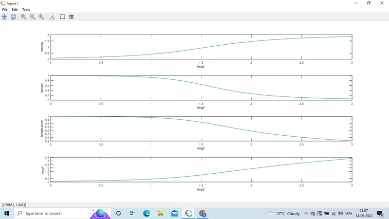
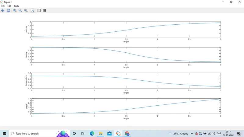
1. Steady-state distribution of primitive variables inside the nozzle
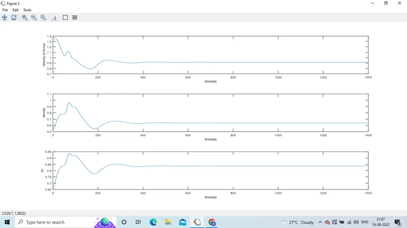
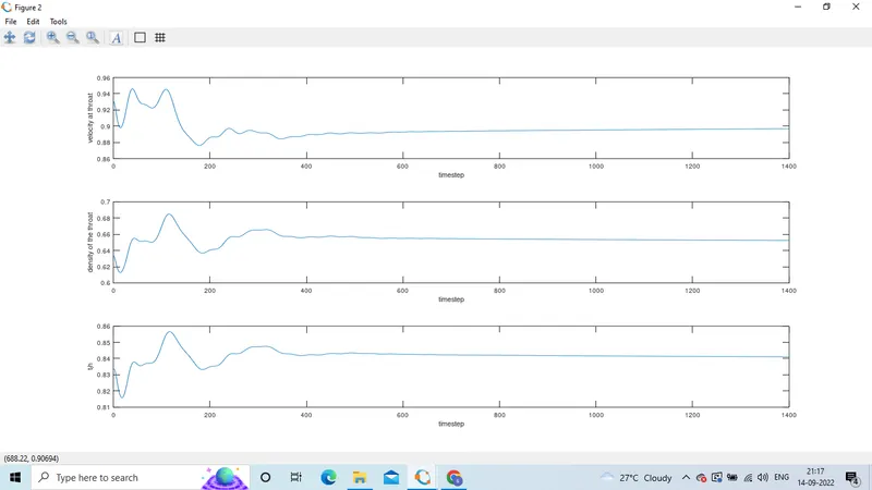
2. Time-wise variation of the primitive variables
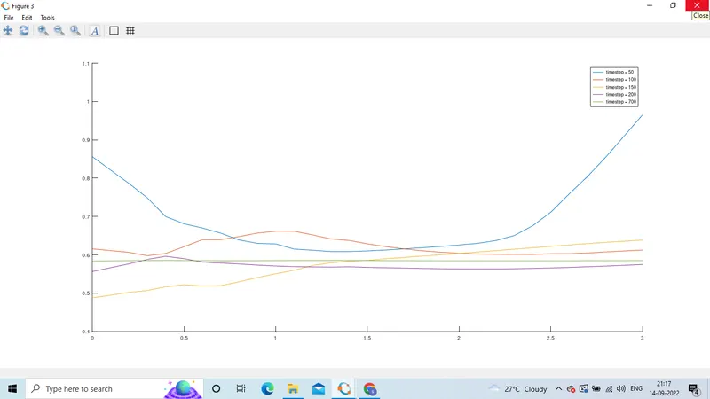
3. Variation of Mass flow rate distribution inside the nozzle at different time steps during the time-marching process
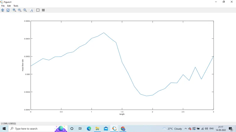
4. Comparison of Normalized mass flow rate distributions of both forms
GOVERNING EQUATIONS:- We have to solve the conservative and non-conservative forms
1. conservative forms has consists of three equations [a]. continuity equation [b]. momentum equation [c]. Energy equation. The conservative method to solve the predictor method and corrector method.
2. Non-conservative forms conservative forms has consists of three equations [a]. continuity equation [b]. momentum equation [c]. Energy equation. The conservative method to solve the predictor method and corrector method.
- Governing equations of the conservative forms:-
- Continuity equation:

Momentum Equation:
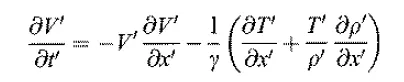
Energy Equation:

-
Continuity equation:
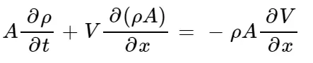
Momentum Equation:
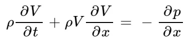
Energy Equation:
Non- conservative form
-
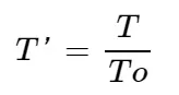
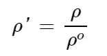
Here the temperature and density are denoted by To and p0 , respectively, we define the nondimensional temperature and density, respectively as
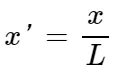
Moreover L denote the length of the nozzle, we define a dimensionless length as
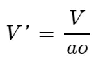
Denoting the speed of sound in the reservoir as 'ao' we define a dimensionless velocity as,
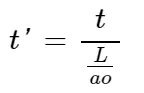
Also, the quantity L/ao has the dimension of time, and we define a dimensionless time as
Finally, we ratio the local area A to the sonic throat area A* and dimensional pressure divided resevoir pressure 'p0' we define a dimensionless area and presure respectively as,

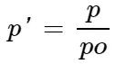
-
Then returning to the governing equations and if we introduce these dimensionless variables we get the non-dimensional governing equations as follows,
Continuity equation:
Momentum Equation:
Energy Equation:
-
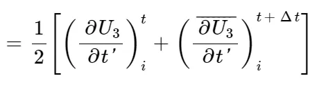
We have calculate the time derivatives by using these updated values by using backward difference.Then the average value of these time derivatives is found out.
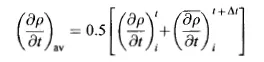
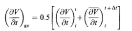
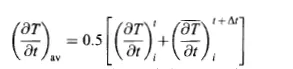
2) Conservative form:
continuity equation :
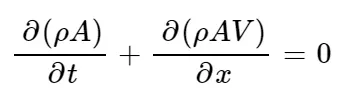
Momentum Equation:
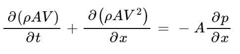
Energy Equation:

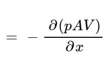
Now converting these equations to non-dimensional form we get the governing equations as
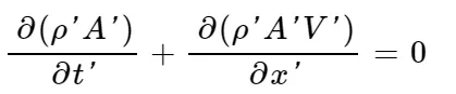
continuity equation :
Momentum Equation:
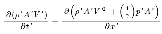
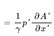
Energy Equation:

Let us express the equations for quasi-onedimensional flow in generic form. Let us define the elements of the solutions vector U, the flux vector F, and the source term J as follows.
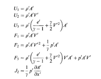
Now substituting these terms in the above governing equations we get,
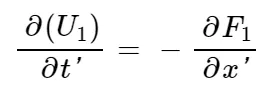
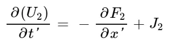
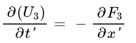
To obtain the primitive variables (p, V, T,p, etc.), we must decode the elements U1, U2, and U3 as follows. From the definitions of U1 , U2 , and U3 given above, we have
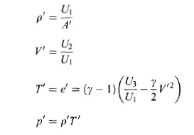
In the above equations, we note that the flux vector elements F1, F2, and F3 and source terms are couched in terms of the primitive variables. When the computer program is written with F 1 , F2 , and F3 expressed directly in terms of p', V', p', and e', instabilities develop during the course of the time-marching solution .So,we write such that the governing equations are in Pure form in terms of the elements of the solution vector i.e, in terms of U1,U2 and U3.
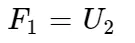
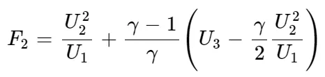
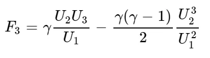

Finally the next step to do is discretization .We take the governing equations that consists of flux terms and source terms and discretize them by using MacCormack's method.
Predictor step:. To start the calculation, we use the initial conditions for U1, U2, and U3 to calculate the initial values of F1, F2, and F3 and and we use these values to calculate the values of U1,U2 and U3 in the next time step .Calculating the time derivatives by using forward difference to the RHS terms to discretize and these time derivatives are used to calculate the predicted values of U1 ,U2 and U3.
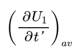
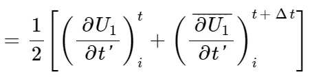
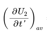
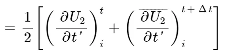
Corrector Step : Now using the predicted values we calculate the new flux terms and source terms .Then we calculate the time derivative terms by using backward difference.Then we calculate the average values of time derivatives of predictor and corrector steps .
MAIN PROGRAM OF THE NON-CONSERVATIVE -FORM: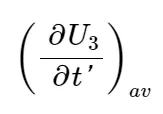
clear all
close all
clc
% inputs
n = 31;
x = linspace(0,3,n);
dx = x(2)-x(1);
% calculate the initial profiles
rho = 1-0.3146*x;
t = 1-0.2314*x;
v = (0.1+1.09*x).*t.^0.5;
gamma = 1.4;
% calculate the area
a = 1+2.2*(x-1.5).^2;
pos = find(a==min(a))
% time steps
nt = 1400;
cfl=0.5;
dt = min(cfl.*dx./(sqrt(t)+v));
% outer time loop
for k = 1:nt
% predictor method
rho_old = rho;
v_old = v;
t_old = t;
for j = 2:n-1
dvdx = (v(j+1)-v(j))/dx;
drhodx = (rho(j+1)-rho(j))/dx;
dtdx = (t(j+1)-t(j))/dx;
dlogadx = (log(a(j+1))-log(a(j)))/dx;
% continuty equation
drhodt_p(j) = -rho(j)*dvdx-rho(j)*v(j)*dlogadx-v(j)*drhodx;
% momentum equation
dvdt_p(j) = -v(j)*dvdx-(1/gamma)*(dtdx+(t(j)/rho(j))*drhodx);
% energy equation
dtdt_p(j) = -v(j)*dtdx-(gamma-1)*t(j)*(dvdx+v(j)*dlogadx);
% solution update
v(j) = v(j)+dvdt_p(j)*dt;
rho(j) = rho(j)+drhodt_p(j)*dt;
t(j) = t(j)+dtdt_p(j)*dt;
end
% corrector method
for j = 2:n-1
dvdx = (v(j)-v(j-1))/dx;
drhodx = (rho(j)-rho(j-1))/dx;
dtdx = (t(j)-t(j-1))/dx;
dlogadx =(log(a(j))-log(a(j-1)))/dx;
% continuty equation
drhodt_c(j) = -rho(j)*dvdx-rho(j)*v(j)*dlogadx-v(j)*drhodx;
% momentum equation
dvdt_c(j) = -v(j)*dvdx-(1/gamma)*(dtdx+(t(j)/rho(j))*drhodx);
% energy equation
dtdt_c(j) = -v(j)*dtdx-(gamma-1)*t(j)*(dvdx+v(j)*dlogadx);
end
% compute the average time derivative
drhodt = 0.5*(drhodt_p+drhodt_c);
dvdt = 0.5*(dvdt_p+dvdt_c);
dtdt = 0.5*(dtdt_p+dtdt_c);
% final solution update
for i = 2:n-1
rho(i) = rho_old(i)+drhodt(i)*dt;
v(i) = v_old(i)+dvdt(i)*dt;
t(i) = t_old(i)+dtdt(i)*dt;
end
% apply the boundary conditions
% inlet
v(1) = 2*v(2)-v(3);
% outlet
v(n) = 2*v(n-1)-v(n-2);
rho(n) = 2*rho(n-1)-rho(n-2);
t(n) = 2*t(n-1)-t(n-2);
rho_th(k) = rho(pos);
t_th(k) = t(pos);
v_th(k) = v(pos);
mdot = rho.*a.*v;
figure(3)
hold on
if k==50
plot(x,mdot)
endif
if k==100
plot(x,mdot)
endif
if k==150
plot(x,mdot)
endif
if k==200
plot(x,mdot)
endif
if k==700
plot(x,mdot,'display','dfasdfa')
endif
end
legend('timestep = 50','timestep = 100','timestep = 150','timestep = 200','timestep = 700')
mach = v./sqrt(t)
figure(1)
subplot(4,1,1)
plot(x,v)
xlabel('length')
ylabel('velocity')
subplot(4,1,2)
plot(x,rho)
xlabel('length')
ylabel('density')
subplot(4,1,3)
plot(x,t)
xlabel('length')
ylabel('temperature')
subplot(4,1,4)
plot(x,mach)
xlabel('length')
ylabel('mach')
figure(2)
subplot(3,1,1)
plot(v_th)
xlabel('timestep')
ylabel('velocity at throat')
subplot(3,1,2)
plot(rho_th)
xlabel('timestep')
ylabel('density')
subplot(3,1,3)
plot(t_th)
xlabel('timestep')
ylabel('t_th')
figure(4)
plot(x,mdot)
xlabel('length')
ylabel('mdot')
OUT-PUT SCREEN SHOTS :-
CASE_1:-
CASE_2:-
CASE_3:-
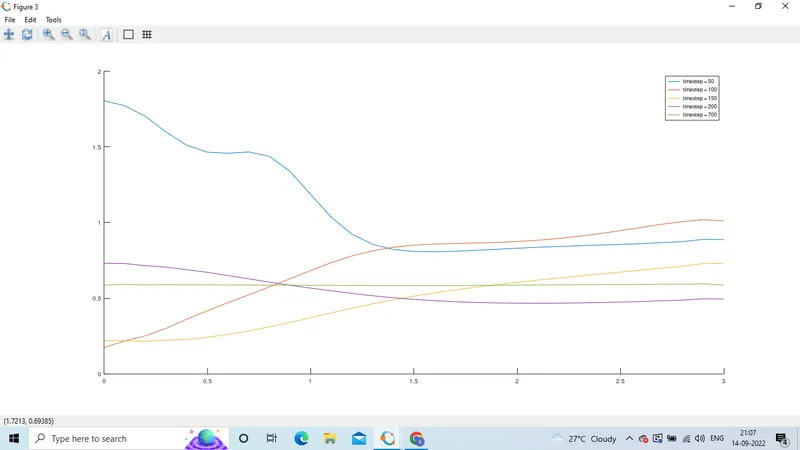
CASE_4:-
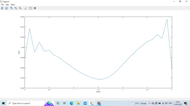
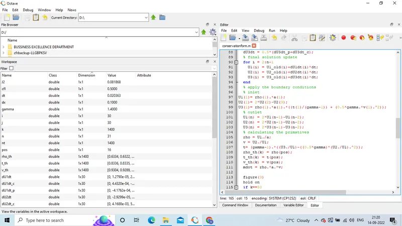
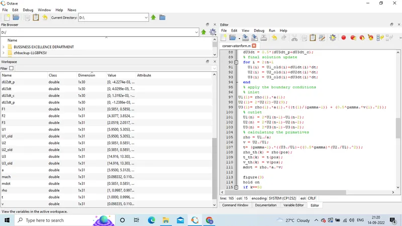
MAIN-PROGRAMME SCREEN SHORT:-
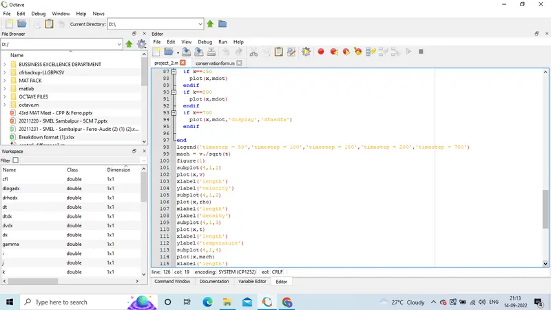
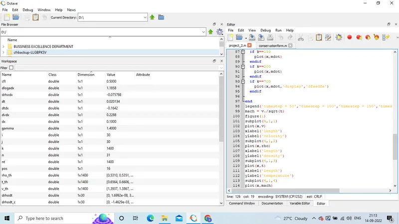
CONSERVATIVE FORM PROGRAMMING:-
clear all
close all
clc
% inputs
n = 31;
x = linspace(0,3,n);
dx = x(2)-x(1);
for i =1:length(x)
if x(i)>=0 && x(i)<=0.5
rho(i) = 1;
t(i)= 1;
elseif x(i)>=0.5 && x(i)<=1.5
rho(i) = 1.0-0.366*(x(i)-0.5);
t(i) = 1.0-0.167*(x(i)-0.5);
elseif x(i)>=1.5 && x(i)<=3.5
rho(i) = 0.634-0.3879*(x(i)-1.5);
t(i) = 0.833-0.3507*(x(i)-1.5);
end
end
gamma = 1.4;
% calculate the area
a = 1+2.2*(x-1.5).^2;
pos = find(a == min(a))
v = 0.59./(rho.*a);
% time steps
nt = 1400;
cfl=0.5;
dt = min(cfl.*dx./(sqrt(t)+v));
% declaring U1 U2 and U3
U1= rho.*a;
U2= rho.*a.*v;
U3= rho.*a.*((t/(gamma-1)) + (0.5*gamma.*v.^2));
% outer time loop
for k = 1:nt
% predictor method
U1_old = U1;
U2_old = U2;
U3_old = U3;
F1= U2;
F2= (U2.^2./U1) + (gamma^-1*(gamma-1)).*(U3-0.5*gamma*(U2.^2./U1));
F3= (gamma*U2.*U3./U1)-(0.5*(gamma^2-gamma)*(U2.^3./U1.^2));
for j = 2:n-1
J2= (1/gamma).*rho(j).*t(j).*(a(j+1)-a(j))/dx;
% continuty equation
dU1dt_p(j) = - (F1(j+1)-F1(j))/dx;
% momentum equation
dU2dt_p(j) = - (F2(j+1)-F2(j))/dx + J2;
% energy equation
dU3dt_p(j) = - (F3(j+1)-F3(j))/dx;
% solution update
U1(j) = U1(j)+dU1dt_p(j)*dt;
U2(j) = U2(j)+dU2dt_p(j)*dt;
U3(j) = U3(j)+dU3dt_p(j)*dt;
end
% update of varibles
rho = U1./a;
t= (gamma-1).*((U3./U1)-((0.5*gamma)*(U2./U1).^2));
v = U2./U1;
% update the flux vector
F1= U2;
F2= (U2.^2./U1) + (gamma^-1*(gamma-1)).*(U3-0.5*gamma*(U2.^2./U1));
F3= (gamma*U2.*U3./U1)-(0.5*(gamma^2-gamma)*(U2.^3./U1.^2));
% corrector method
for j = 2:n-1
J2= (1/gamma).*rho(j).*t(j).*(a(j)-a(j-1))/dx;
% continuty equation
dU1dt_c(j) = - (F1(j)-F1(j-1))/dx;
% momentum equation
dU2dt_c(j) = - (F2(j)-F2(j-1))/dx + J2;
% energy equation
dU3dt_c(j) = - (F3(j)-F3(j-1))/dx;
end
% compute the average time derivative
dU1dt = 0.5*(dU1dt_p+dU1dt_c);
dU2dt = 0.5*(dU2dt_p+dU2dt_c);
dU3dt = 0.5*(dU3dt_p+dU3dt_c);
% final solution update
for i = 2:n-1
U1(i) = U1_old(i)+dU1dt(i)*dt;
U2(i) = U2_old(i)+dU2dt(i)*dt;
U3(i) = U3_old(i)+dU3dt(i)*dt;
end
% apply the boundary conditions
% inlet
U1(1)= rho(1).*a(1);
U2(1)= 2*U2(2)-U2(3);
U3(1)= rho(1).*a(1).*((t(1)/(gamma-1)) + (0.5*gamma.*v(1).^2));
% outlet
U1(n) = 2*U1(n-1)-U1(n-2);
U2(n) = 2*U2(n-1)-U2(n-2);
U3(n) = 2*U3(n-1)-U3(n-2);
% calculating the primatives
rho = U1./a;
v = U2./U1;
t= (gamma-1).*((U3./U1)-((0.5*gamma)*(U2./U1).^2));
rho_th(k) = rho(pos);
t_th(k) = t(pos);
v_th(k) = v(pos);
mdot = rho.*a.*v;
figure(3)
hold on
if k==50
plot(x,mdot)
endif
if k==100
plot(x,mdot)
endif
if k==150
plot(x,mdot)
endif
if k==200
plot(x,mdot)
endif
if k==700
plot(x,mdot,'display','dfasdfa')
endif
end
legend('timestep = 50','timestep = 100','timestep = 150','timestep = 200','timestep = 700')
mach = v./sqrt(t)
figure(1)
subplot(4,1,1)
plot(x,v)
xlabel('length')
ylabel('velocity')
subplot(4,1,2)
plot(x,rho)
xlabel('length')
ylabel('density')
subplot(4,1,3)
plot(x,t)
xlabel('length')
ylabel('temperature')
subplot(4,1,4)
plot(x,mach)
xlabel('length')
ylabel('mach')
figure(2)
subplot(3,1,1)
plot(v_th)
xlabel('timestep')
ylabel('velocity at throat')
subplot(3,1,2)
plot(rho_th)
xlabel('timestep')
ylabel('density of the throat')
subplot(3,1,3)
plot(t_th)
xlabel('timestep')
ylabel('t_th')
figure(4)
plot(x,mdot)
xlabel('length')
ylabel('mass flow rate')
OUTPUTS:-
CASE_1:-
CASE_2;
CASE_3:-
CASE_4:-
MAIN PROGRAM OUTPUT:-