Week 3 - Solving second order ODEs

SECOND ORDER DIFFERENTIAL EQUATION BY USING SIMPLE PENDULUM:-

d^2(theta)/dt^2 + b/m .d(theta)/dt + g/l + sin(theta) = 0......... [1].

b = damping factor

m = mass

g = gravity

theta = theta1..........[2].

d(theta)/dt = d(theta1)/dt = theta2.......[3].

d^2(theta)/dt^2 = d^2(theta1)/dt^2 = d/dt(dtheta1/dt) = d/dt(theta2).........[4].

d^2theta/dt^2 + b/m.dtheta/dt + g/l sin(theta)...............[5].

d^2theta1/dt^2 + b/m .dtheta1/dt +g/l sin(theta1)..........[6].

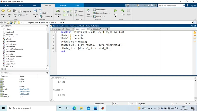
d(theta1)/dt = theta2 , dtheta2/dt = -b/m.theta2-g/lsin(theta1).........[7].

d/dt[theta1; theta2] = [theta2; -b/m theta2-g/lsin(theta).........[8].

EXPLANATION OF SIMPLE PENDULUM CODE:-

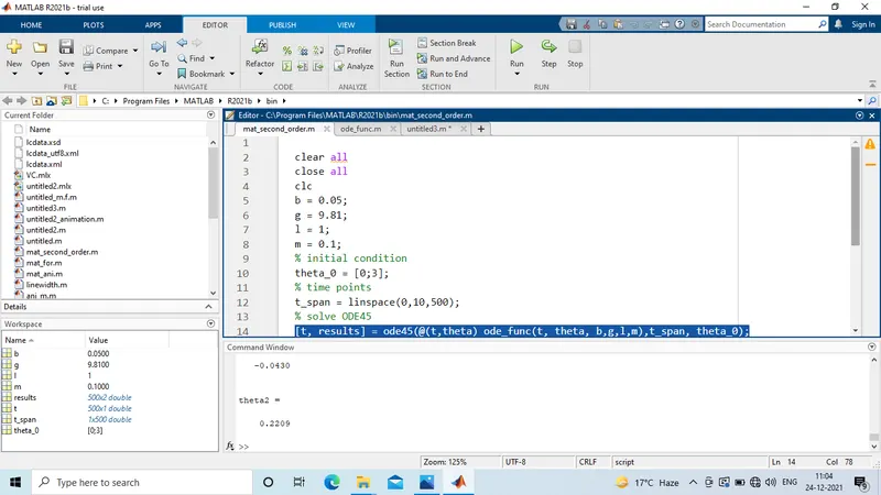
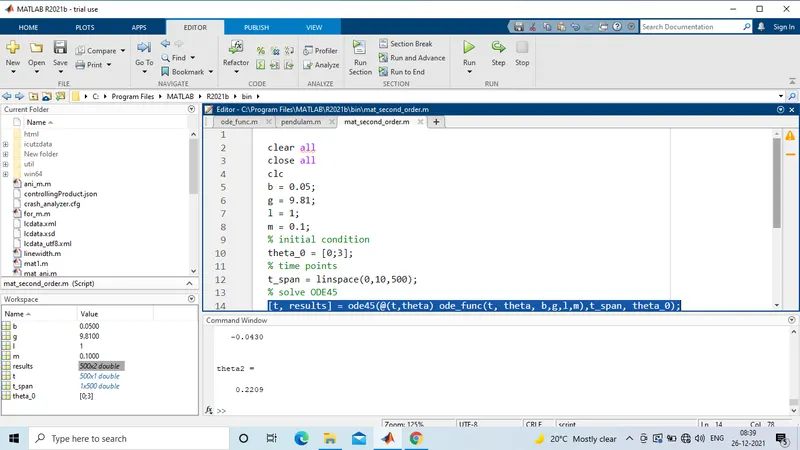
b = 0.05; %damping factor

g = 9.81; %acceleration due to gravity m^2/sec

l = 1;% length of the pendulum

m = 0.1; % mass of pendulum in kg

t_span = linspace(0,10,500); % time in array

theta_0 = [0;3] % initial conditions - angular displacement, velocity

t = [0,20];

% solving ordinary differential equation by ode45

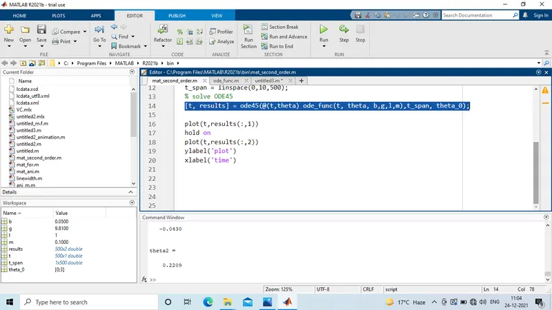
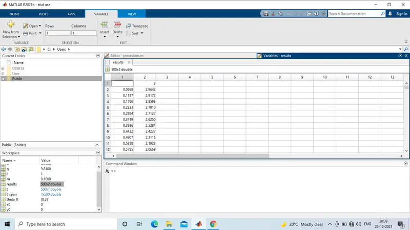
[t, results] = ode45(@(t,theta) ode_func(t, theta, b,g,l,m),t_span, theta_0);

in this equation

ode_45 = inbuilt

(@(t,theta) =% dependent and independent varible

ode_func(t, theta, b,g,l,m) = %input parameters

theta_0 = %initial conditions

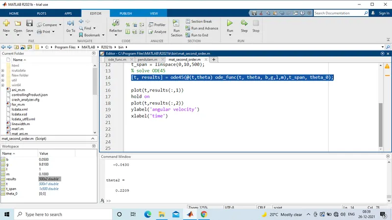
% plotting graphs

plot(t, results(:,1))

hold on

plot(t, results(:,2))

y label ('plot')

x label ('time')

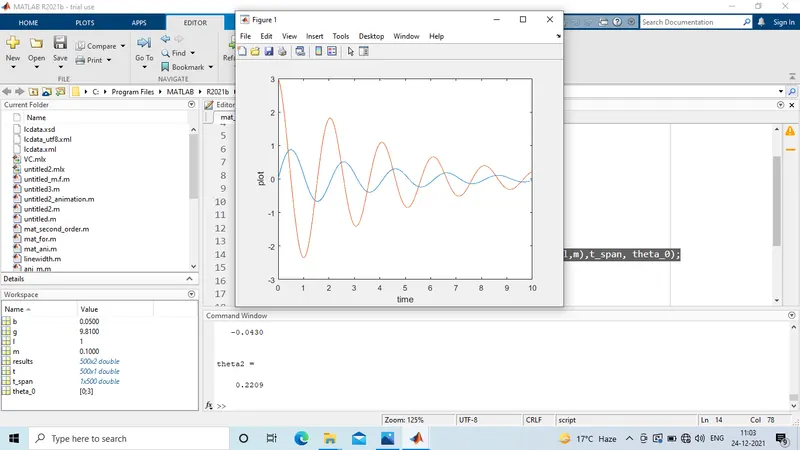
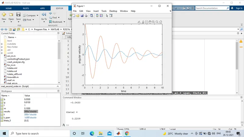
% in first graph we have take x- axis = time , angular displacement = y-axis

% in second graph we have take x- axis = time, angular velocity = y-axis

simple pendulum codes:-