Week 3.5 - Deriving 4th order approximation of a 2nd order derivative using Taylor Table method
AIM :- To write a program for in octave for fourth order approximation second order derivative by the following methods.
1. central difference
2. skewed right side difference.
3. skewed left side difference.
objective:- To evaluate the second order derivative f(x) = exp(x) cosx, using above mentioned order of approximations
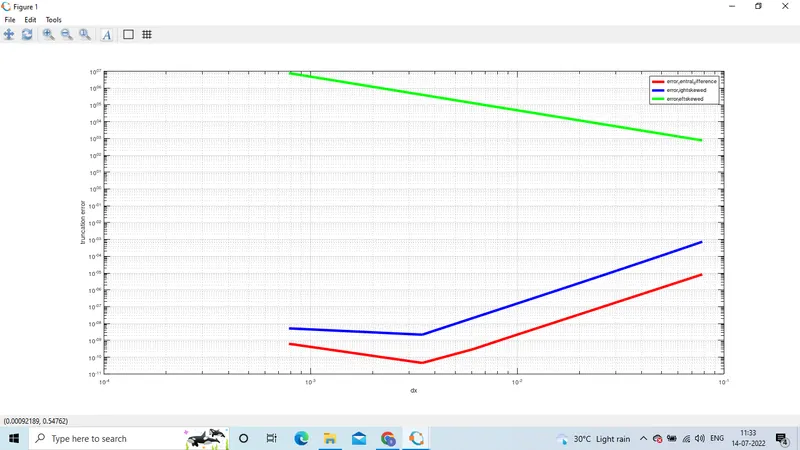
# To plot and comapre the values and errors of 3 merthods derived.
Findings:-
1. x = pi/3
2. dx = linspace(pi/40,pi/4000,30)
3. C = rats(inv(A)*B)......... [FOR CENTRAL DIFFERENCE] % Dismal values convert in fractional values.
4. R = rats(inv(P)*Q).........[FOR LEFT SIDE SKEME].
5. U = rats(inv(S)*T)............ [FOR RIGHT SIDE SKEME].
6. dr_ central(i)
7. error_central_difference(i)
8. dr_rightskwed
9. error_rightskwed(i)
10. dr_leftskwed(i)
11. error_leftskwed(i)
12. FUNCTION F(X) = exp(x)*cos(x)
13. analytical derivative = -2*exp(x)*sin(x)
THEORY :-
1. CENTRAL DIFFERENCE:- Here the nodes are we selected are symetrically that is in the data taken from both sides of point.
`del^2f`/ `delx^2` = af(i-2)+bf(i-1)+cf(i)+df(i+1)+ef(i+2)............................central_difference
f(x) dx f^1(x) dxf^11(x) dxf^111(x) dxf^1111(x)
af(i-1) a -2a 4a/2 -8/6 16a/24
bf(i-2) b -b b/2 -b/6 b/24
cf(i) c 0 0 0 0
df(i+1) d d d/2 d/6 d/24
ef(i+2) e 2e 4e/2 8e/6 16e/24
af(i-2)+bf(i-1)+cf(i)+df(i+1)+ef(i+2) = 0 0 1 0 0.................... co-efficients of central_difference
2. skwed right side difference:- When the data point of the left nodes are not avaible then we have to rely on the avaiable data.
f(x) dx dx(f^1(x) dx(f^11(x) dx(f^111(x)) dx(f^1111(x))
af(i) a 0 0 0 0 0
bf(i+1) b b b/2 b/6 b/24 b/120
cf(i+2) c 2c 4c/2 8c/6 16c/24 32c/120
df(i+3) d 3d 9d/2 27d/6 81d/24 243d/120
ef(i+4) e 4e 16e/2 64e/6 256e/24 1024e/120
ff(i+5) f 5f 25f/2 125f/6 625f/24 3125f/120
af+bf(i+1)+cf(i+2)+df(i+3)+ef(i+4)+ff(i+5) = 0 0 1 0 0 0 ............... co-efficients of right skwed.
3. Left hand skewe difference:-
af(i-5) a -5a 25a/2 -125a/6 625a/24 -3125a/120
bf(i-4) b -4b 16b/2 -64b/6 256b/24 -1024b/120
cf(i-3) c -3c 9c/2 -27c/6 81c/24 -243c/120
df(i-2) d -2d 4d/2 -8d/6 16d/24 -32d/120
ef(i-1) e -e e/2 -e/6 e/24 -e/120
ff(i) f 0 0 0 0 0
CENTRAL DIFFERENCE CO-EFFICIENTS:-
% for central_differencing value of co-efficients
A = [1 1 1 1 1;-2 -1 0 1 2;2 1/2 0 1/2 2;-8/6 -1/6 0 1/6 8/6;16/24 1/24 0 1/24 16/24];
B = [0;0;1;0;0];
C = rats(inv(A)*B);
% co-efficients values of cental_differencing
a = -1/12;
b = 4/3;
c = -5/2;
d = 4/3;
e = -1/12;
% for left_hand_skewed scheme
P = [1 1 1 1 1 1;-5 -4 -3 -2 -1 0;25/2 8 9/2 4/2 1/2 0;-125/6 -64/6 -27/6 -8/6 -1/6 0;625/24 256/24 81/24 16/24 1/24 0;-3125/120 -1024/120 -243/120 -32/120 -1/120 0];
Q = [0;0;1;0;0;0];
R = rats(inv(P)*Q);
% co-efficients values of left_hand_skwed scheme
a1 = -5/6;
b1 = 61/12;
c1 = -13;
d1 = 107/6;
e1 = -77/6;
f1 = 15/4;
% for right_hand_skewed scheme
S = [1 1 1 1 1 1;0 1 2 3 4 5;0 1/2 2 9/2 8 25/2;0 1/6 8/6 27/6 64/6 125/6;0 1/24 16/24 81/24 256/24 625/24;0 1/120 32/120 243/120 1024/120 3125/120];
T = [0;0;1;0;0;0];
U = rats(inv(S)*T);
% co-efficients values of right_hand_skwed scheme
a2 = 15/4;
b2 = -77/6;
c2 = 107/6;
d2 = -13;
e2 = 61/12;
f2 = -5/6;
OCTAVE CODE:-
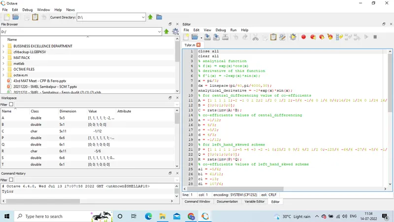
close all
clear all
% analytical function
% f(x) = exp(x)*cos(x)
% derivative of this function
% f^1(x) = -2exp(x)*sin(x);
x = pi/3;
dx = linspace(pi/40,pi/4000,30);
analytical_derivative = -2*exp(x)*sin(x);
% for central_differencing value of co-efficients
A = [1 1 1 1 1;-2 -1 0 1 2;2 1/2 0 1/2 2;-8/6 -1/6 0 1/6 8/6;16/24 1/24 0 1/24 16/24];
B = [0;0;1;0;0];
C = rats(inv(A)*B);
% co-efficients values of cental_differencing
a = -1/12;
b = 4/3;
c = -5/2;
d = 4/3;
e = -1/12;
% for left_hand_skewed scheme
P = [1 1 1 1 1 1;-5 -4 -3 -2 -1 0;25/2 8 9/2 4/2 1/2 0;-125/6 -64/6 -27/6 -8/6 -1/6 0;625/24 256/24 81/24 16/24 1/24 0;-3125/120 -1024/120 -243/120 -32/120 -1/120 0];
Q = [0;0;1;0;0;0];
R = rats(inv(P)*Q);
% co-efficients values of left_hand_skwed scheme
a1 = -5/6;
b1 = 61/12;
c1 = -13;
d1 = 107/6;
e1 = -77/6;
f1 = 15/4;
% for right_hand_skewed scheme
S = [1 1 1 1 1 1;0 1 2 3 4 5;0 1/2 2 9/2 8 25/2;0 1/6 8/6 27/6 64/6 125/6;0 1/24 16/24 81/24 256/24 625/24;0 1/120 32/120 243/120 1024/120 3125/120];
T = [0;0;1;0;0;0];
U = rats(inv(S)*T);
% co-efficients values of right_hand_skwed scheme
a2 = 15/4;
b2 = -77/6;
c2 = 107/6;
d2 = -13;
e2 = 61/12;
f2 = -5/6;
f = @(x)exp(x)*cos(x);
for i = 1:1:length(dx)
dr_central(i) = (a*f(x-2*dx(i))+b*f(x-1*dx(i))+c*f(x)+d*f(x+1*dx(i))+e*f(x+2*dx(i)))/(dx(i)^2);
error_central_difference(i) = abs(analytical_derivative- dr_central(i));
dr_rightskwed(i) = (a2*f(x)+b2*f(x+1*dx(i))+c2*f(x+2*dx(i))+d2*f(x+3*dx(i))+e2*f(x+4*dx(i))+f2*f(x+5*dx(i)))/(dx(i)^2);
error_rightskwed(i) = abs(analytical_derivative- dr_rightskwed(i));
dr_leftskwed(i) = (a1*f(x-5*dx(i))+b1*f(x-4*dx(i))+c1*f(x-3*dx(i))+d1*f(x-2*dx(i))+e1*f(x-1*dx(i))+f(1*f(x)))/(dx(i)^2);
error_leftskwed(i) = abs(analytical_derivative- dr_leftskwed(i));
endfor
figure(1)
loglog (dx,error_central_difference,'linewidth',3,'color','r')
hold on
loglog (dx,error_rightskwed,'linewidth',3,'color','b')
hold on
loglog (dx,error_leftskwed,'linewidth',3,'color','g')
xlabel('dx')
ylabel('truncation error')
legend('error_central_difference','error_rightskewed','error_leftskewed')
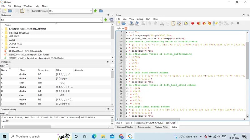
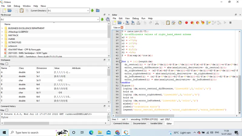
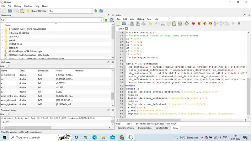
OCTAVE CODE SCREEN SHORTS:-
GRAPHS OF 3- SCHEMES:-