Week 7 - Simulation of a 1D Super-sonic nozzle flow simulation using Macormack Method
Theory:
Introduction:Direct numerical stimulation of fluid flow through nozzle has always been a challenging problem and an area of immense interest for modern engineers. Converging-Diverging nozzle has been extensively used in a wide range of Industrial
applications ranging from steam turbines to rocket engine nozzles.
The condition for operation so that the nozzle produces supersonic flow is that the Mach number at throat should be equal to one. This condition is known as choked flow. As the fluid expands further in the diverging section, the fluid flow increases to supersonic velocities.(Mach Number>1).If the choke condition is not met, the nozzle simply acts as a Venturi tube and would produce subsonic flow even at the outlet. This paper uses an explicit finite difference scheme for numerical solution of fluid flow. This scheme is fully explicit and second order accurate in both time and space.
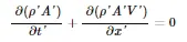
for non consevation form:
continuty equation :

momentum equation

energy equation

for coservation form:
continuty equation
momentum equation

energy equation

Maccarmack method:In CFD, the MacCormack method is a widely used discretization scheme for the numerical solution of hyperbolic PDE. This second-order FDM was introduced by Robert W. MacCormack in 1969.The MacCormack method is elegant and easy to understand and program.
The MacCormack method is a variation of the two step Lax Wendroff but is much simpler in application. To illustrate the algorithm, consider the following first order hyperbolic equation.
% witting program for simulation of 1D NOZZLE SUPERSONIC FLOW USING MACCORMAC'S METHOD

clear all
close all
clc

%defing the inputs
%number of grids points

n=31;
x=linspace(0,3,n);
dx=x(2)-x(1);


gamma=1.4;

%numbers of time steps

nt=1400;
CFL=0.5;

%defing the function for non conservation form of simulation

tic;
[mass_flow_rate_nc, presure_nc, mach_num_nc, rho_nc, v_nc, T_nc, rho_trottle_nc, v_trottle_nc, T_trottle_nc, mass_flow_rate_trottle_nc, presure_trottle_nc, mach_num_trottle_nc]=non_conservative_form_original(x,dx,n,gamma,nt,CFL)
time_elapsed=toc;
fprintf('time elapesed for non coservation form:%f',time_elapsed)
hold on

%ploting the graphs

figure(3)

%for density

subplot(4,1,1)
plot(linspace(1,nt,1400),rho_trottle_nc,"Color","m");
ylabel("density")
legend({'density at trottle'})
title('timestep variation at trottle area-non conservation form')

%for tempreture

subplot(4,1,2)
plot(linspace(1,nt,1400),T_trottle_nc,"Color","b");
ylabel("tempreture")
legend({'tempreture at trottle'})
title('timestep variation at trottle area-non conservation form')

% for presure

subplot(4,1,3)
plot(linspace(1,nt,1400),presure_trottle_nc,"Color","r");
ylabel("presure")
legend({'presure at trottle'})
title('timestep variation at trottle area-non conservation form')

%for mach number

subplot(4,1,4)
plot(linspace(1,nt,1400),mach_num_trottle_nc,"Color","m");
xlabel('time step')
ylabel("mach nuber")
legend({'mach num at trottle'})
title('timestep variation at trottle area-non conservation form')


% steady sTATE simulation for primitive value for nom conservation form

figure(4)

%for density

subplot(4,1,1)
plot(x,rho_nc,"Color","m");
ylabel("density")
legend({'density'})
title('timestep variation at trottle area-non conservation form')

%for tempreture

subplot(4,1,2)
plot(x,T_nc,"Color","b");
ylabel("tempreture")
legend({'tempreture'})
title('timestep variation at trottle area-non conservation form')

% for presure

subplot(4,1,3)
plot(x,presure_nc,"Color","r");
ylabel("presure")
legend({'presure'})
title('timestep variation at trottle area-non conservation form')

%for mach number

subplot(4,1,4)
plot(x,rho_nc,"Color","m");
xlabel('nozzel lenth')
ylabel("mach nuber")
legend({'mach num at trottle'})
title('timestep variation at trottle area-non conservation form')

%defing the function for conservation form of simulation

tic;
[mass_flow_rate_c, presure_c, mach_num_c, rho_c,v_c, T_c, rho_trottle_c, v_trottle_c, T_trottle_c, mass_flow_rate_trottle_c, presure_trottle_c, mach_num_trottle_c]=conservation_form(x,dx,n,gamma,nt,CFL);
time_elapsed_c=toc;
fprintf('time elapesed for coservation form:%f',time_elapsed_c)
hold on

%plotting

figure(5)

%for density

subplot(4,1,1)
plot(linspace(1,nt,1400),rho_trottle_c,'Color','m');
ylabel("density")
legend({'density at trottel'})
title('timestep variation at trottle area- conservation form')

%for tempreture

subplot(4,1,2)
plot(linspace(1,nt,1400),T_trottle_c,'Color',"b");
ylabel("tempreture")
legend({'tempreture at trottle'})
title('timestep variation at trottle area- conservation form')

% for presure

subplot(4,1,3)
plot(linspace(1,nt,1400),presure_trottle_c,"Color","r");
ylabel("presure")
legend({'presure at trottle'})
title('timestep variation at trottle area- conservation form')

%for mach number

subplot(4,1,4)
plot(linspace(1,nt,1400),mach_num_trottle_c,"Color","m");
xlabel('time step')
ylabel("mach nuber")
legend({'mach num at trottle'})
title('timestep variation at trottle area- conservation form')


% steady sTATE simulation for primitive value for nom conservation form

figure(6)

%for density

subplot(4,1,1)
plot(x,rho_c,"Color","m");
ylabel("density")
legend({'density'})
title('timestep variation at trottle area- conservation form')


%for tempreture

subplot(4,1,2)
plot(x,T_c,"Color","b");
ylabel("tempreture")
legend({'tempreture'})
title('timestep variation at trottle area-conservation form')

% for presure

subplot(4,1,3)
plot(x,presure_c,"Color","r");
ylabel("presure")
legend({'presure'})
title('timestep variation at trottle area- conservation form')

%for mach number

subplot(4,1,4)
plot(x,mach_num_c,"Color","m");
xlabel('nozzel lenth')
ylabel("mach nuber")
legend({'mach num at trottle'})
title('timestep variation at trottle area- conservation form')


%camparing the plots of narmalization mass flow rate of both forms

figure(7)
hold on
plot(x,mass_flow_rate_nc,'r','linewidth',2)
hold on
plot(x,mass_flow_rate_c,'b','linewidth',2)
hold on
grid on
legend('non conversion','conversion')
xlabel('lenght of the domain')
ylabel('mass flow rate')
title('camparison of narmalization mass flow rate of both forms')
Function for Conservation Form
%writting the function for non conservation form using maccormack method

function [mass_flow_rate_c, presure_c, mach_num_c, rho_c, v_c, T_c, rho_trottle_c, v_trottle_c, T_trottle_c, mass_flow_rate_trottle_c, presure_trottle_c, mach_num_trottle_c]=conservation_form(x,dx,n,gamma,nt,CFL)

%[mass_flow_rate_c, presure_c, mach_num_c, rho_c, v_c, T_c, rho_trottle_c, v_trottle_c, T_trottle_c, mass_flow_rate_trottle_c, presure_trottle_c, mach_num_trottle_c]=conservation_form(x,dx,n,gamma,nt,CFL);

%defining the intial boundry condition for density and tempreture

for m =1:n
    if(x(m) >=0 && x(m) <=0.5)
        rho_c(m)=1;
        T_c(m) =1;
    elseif (x(m) >=0.5 && x(m) <=1.5)
        rho_c(m)=1-0.366*(x(m)-0.5);
        T_c(m) =1-0.167*(x(m)-0.5);
    elseif  (x(m) >=1.5 && x(m) <=3.5)
         rho_c(m)=0.634-0.3879*(x(m)-1.5);
        T_c(m) =0.833-0.3507*(x(m)-1.5);
    end
end

%defining for velocity

a=1+2.2*(x-1.5).^2;
v_c =0.59./(rho_c.*a);
presure_c=rho_c.*T_c;

% defining the trottle

trottle = find(a==1);

% defing the initiel solution variabels

U1 =rho_c.*a;
U2 =rho_c.*a.*v_c;
U3 =rho_c.*a.*(T_c./(gamma-1))+((gamma/2).*v_c.^2);

%defining the time loop


for k =1:nt

    %defining the time step

    dt =min(CFL.*dx./(sqrt(T_c)+v_c));

    %defing the old values

    U1_old=U1;
    U2_old=U2;
    U3_old=U3;

    %calculating the flux

    F1=U2;
    F2=((U2.^2)./U1)+((gamma-1)/gamma)*(U3-(gamma/2)*((U2.^2)./U1));
    F3=((gamma*U2.*U3)./U1)-(gamma*(gamma-1)*((U2.^3)./(2*U1.^2)));

    % calculatinf the predector method

    for j = 2:n-1

        % calculating the souse term

        J2(j)=(1/gamma)*rho_c(j)*T_c(j)*((a(j+1)-a(j))/dx);

        % continuty eqution

        dU1_dt_p(j)=-((F1(j+1)-F1(j))/dx);

        % momentum equation

         dU2_dt_p(j)=-((F2(j+1)-F2(j))/dx)+J2(j);


         %energy equation

          dU3_dt_p(j)=-((F3(j+1)-F3(j))/dx);

          % updating the soluton vector

          U1(j)=U1(j)+dU1_dt_p(j)*dt;
          U2(j)=U2(j)+dU2_dt_p(j)*dt;
          U3(j)=U3(j)+dU3_dt_p(j)*dt;
    end

    %updating the flux

    F1=U2;
    F2=((U2.^2)./U1)+((gamma-1)/gamma)*(U3-(gamma*0.5*(U2.^2)./U1));
    F3=((gamma*U2.*U3)./U1)-((gamma*0.5*(gamma-1)*(U2.^3)./(U1.^2)));


    % know calculating for corrector method

    for j=2:n-1

% calculating the souse term

        J2(j)=(1/gamma)*rho_c(j)*T_c(j)*((a(j)-a(j-1))/dx);

        % continuty eqution

        dU1_dt_c(j)=-((F1(j)-F1(j-1))/dx);

        % momentum equation

         dU2_dt_c(j)=-((F2(j)-F2(j-1))/dx)+J2(j);


         %energy equation

          dU3_dt_c(j)=-((F3(j)-F3(j-1))/dx);

    end

    %computing the avarege value

    dU1_dt_av=0.5*(dU1_dt_p+dU1_dt_c);
    dU2_dt_av=0.5*(dU2_dt_p+dU2_dt_c);
    dU3_dt_av=0.5*(dU3_dt_p+dU3_dt_c);

    % calculating the final solution

    for m=2:n-1
        U1(m)=U1_old(m)+dU1_dt_av(m)*dt;
        U2(m)=U2_old(m)+dU2_dt_av(m)*dt;
        U3(m)=U3_old(m)+dU3_dt_av(m)*dt;
    end

    %appliying the boundry conditions at inlets

    U1(1)=rho_c(1)*a(1);
    U2(1)=2*U2(2)-U2(3);
    v_c(1)=U2(1)./U1(1);
    U3(1)=U1(1)*((T_c(1)/(gamma-1))+((gamma/2)*(v_c(1)).^2));

    %at outlet

     U1(n)=2*U1(n-1)-U1(n-2);
     U2(n)=2*U2(n-1)-U2(n-2);
     U3(n)=2*U3(n-1)-U3(n-2);

     %final primitive value update

     rho_c=U1./a;
     v_c=U2./U1;
     T_c=(gamma-1)*((U3./U1)-(gamma/2)*(v_c).^2);

     % defing the mass flow rate

        %defing the flow rate

        mass_flow_rate_c = rho_c.*a.*v_c;
        presure_c = rho_c.*T_c;
        mach_num_c = (v_c./sqrt(T_c));

        % calculating the variables at trottle

        rho_trottle_c(k) = rho_c(trottle);
        T_trottle_c(k) = T_c(trottle);
        v_trottle_c(k) = v_c(trottle);
        mass_flow_rate_trottle_c(k) =  mass_flow_rate_c(trottle);
        presure_trottle_c(k) = presure_c(trottle);
        mach_num_trottle_c(k) = mach_num_c(trottle);

         %comparing the non dimensional mass flow at different time step
         %plotting

         figure(2);

        if  k == 50
             plot(x,mass_flow_rate_c,'b','linewidth',1)
             hold on

        elseif k == 150
              plot(x,mass_flow_rate_c,'c','linewidth',1)
          hold on

        elseif k == 200
             plot(x,mass_flow_rate_c,'k','linewidth',1)
          hold on

        elseif k == 400
             plot(x,mass_flow_rate_c,'g','linewidth',1)
           hold on

        elseif k == 800
             plot(x,mass_flow_rate_c,'m','linewidth',1)
             hold on
        end

end
%labeling
xlabel('domain')
ylabel('mass flow rate conservation')
title('camparing the non dimensinal mass flow rate at diffrent time steps-conservation form ')
legend({'50th time step','150th time step','200th time step','400th time step','800th time step'})
grid on
Function for non conservation form
%writting the function for non conservation form using maccormack method

function [mass_flow_rate_nc, presure_nc, mach_num_nc, rho_nc, v_nc, T_nc, rho_trottle_nc, v_trottle_nc, T_trottle_nc, mass_flow_rate_trottle_nc, presure_trottle_nc, mach_num_trottle_nc]=non_conservative_form_original(x,dx,n,gamma,nt,CFL)


%defining the intial boundry condition

rho_nc=1 - 0.3146*x;
T_nc =1 - 0.2341*x;
v_nc=(0.1+1.09*x).*T_nc.^0.5;

%area of the nozzel

a = 1+2.2*(x-1.5).^2;

% defining trottle
trottle = find(a==1);

%defining the time loop
%defining the nodes

for k =1:nt
    dt =min(CFL.*dx./(sqrt(T_nc)+v_nc));

    %defining the old values

    rho_old=rho_nc;
    T_old=T_nc;
    v_old =v_nc;

    %know we have to solve  for predictor method

    for j =2:n-1


        % simplifying the speciel terms there fore we have equation for continity
         momentum energy in that equation we are descritizing using forword scheme
        dv_dx =(v_nc(j+1)-v_nc(j))./dx;
        drho_dx =(rho_nc(j+1)-rho_nc(j))./dx;
        dT_dx =(T_nc(j+1)-T_nc(j))./dx;
        dlog_a_dx =(log(a(j+1))-log(a(j)))./dx;

        % continuty equation
        drho_dt_p(j)=-rho_nc(j)*dv_dx-rho_nc(j)*v_nc(j)*dlog_a_dx-v_nc(j)*drho_dx;

        %momemtum equation

        dv_dt_p(j)=-v_nc(j)*dv_dx-(1/gamma)*(dT_dx+(T_nc(j)*drho_dx/rho_nc(j)));

        % energy equation
        dT_dt_p(j)=-v_nc(j)*dT_dx-(gamma-1)*T_nc(j)*(dv_dx+v_nc(j)*dlog_a_dx);

        % updating the solution
        rho_nc(j)=rho_nc(j)+drho_dt_p(j)*dt;
        v_nc(j)=v_nc(j)+dv_dt_p(j)*dt;
        T_nc(j)=T_nc(j)+dT_dt_p(j)*dt;
    end

    %know we have to define the equations fo corrector methods
    % simplifying the speciel terms there fore we have equation for continity momentum energy in that equation we are descritizing using backword scheme

    for j=2:n-1
        dv_dx =(v_nc(j)-v_nc(j-1))./dx;
        drho_dx =(rho_nc(j)-rho_nc(j-1))./dx;
        dT_dx =(T_nc(j)-T_nc(j-1))./dx;
        dlog_a_dx =(log(a(j))-log(a(j-1)))./dx;

        % continuty equation

        drho_dt_c(j)=-rho_nc(j)*dv_dx-rho_nc(j)*v_nc(j)*dlog_a_dx-v_nc(j)*drho_dx;

        %momemtum equation

        dv_dt_c(j)=-v_nc(j)*dv_dx-(1/gamma)*(dT_dx+(T_nc(j)*drho_dx/rho_nc(j)));

        % energy equation

        dT_dt_c(j)=-v_nc(j)*dT_dx-(gamma-1)*T_nc(j)*(dv_dx+v_nc(j)*dlog_a_dx);
    end


        % computing the averege vtime deravetion or averege solution

        drho_dt_av =0.5.*(drho_dt_p+drho_dt_c);
        dv_dt_av =0.5.*(dv_dt_p+dv_dt_c);
        dT_dt_av =0.5.*(dT_dt_p+dT_dt_c);

        % final solution

        for m=2:n-1
            rho_nc(m)=rho_old(m)+(drho_dt_av(m))*dt;
            v_nc(m)=v_old(m)+(dv_dt_av(m))*dt;
            T_nc(m)=T_old(m)+(dT_dt_av(m))*dt;
        end

        % applying the boundary conditions
        % At inlet

        rho_nc(1)=1;
        v_nc(1)=2*v_nc(2)-v_nc(3);
        T_nc(1)=1;

        % At oulet
        rho_nc(n)=2*rho_nc(n-1)-rho_nc(n-2);
        v_nc(n)=2*v_nc(n-1)-v_nc(n-2);
        T_nc(n)=2*T_nc(n-1)-T_nc(n-2);

        %defining the flow rate

        mass_flow_rate_nc=rho_nc.*a.*v_nc;
        presure_nc=rho_nc.*T_nc;
        mach_num_nc=(v_nc./sqrt(T_nc));

        % calculating the variables at trottle
        %trottle=find(a==1);

        rho_trottle_nc(k) = rho_nc(trottle);
        T_trottle_nc(k) = T_nc(trottle);
        v_trottle_nc(k) = v_nc(trottle);
        mass_flow_rate_trottle_nc(k) = mass_flow_rate_nc(trottle);
        presure_trottle_nc(k) = presure_nc(trottle);
        mach_num_trottle_nc(k) = mach_num_nc(trottle);

         %comparing the non dimensional mass flow at different time step
         %plotting

         figure(1);

        if  k == 50
             plot(x,mass_flow_rate_nc,'b','linewidth',1)
             hold on

        elseif k == 150
              plot(x,mass_flow_rate_nc,'c','linewidth',1)


        elseif k == 200
             plot(x,mass_flow_rate_nc,'m','linewidth',1)


        elseif k == 400
             plot(x,mass_flow_rate_nc,'r','linewidth',1)


        elseif k == 800
             plot(x,mass_flow_rate_nc,'k','linewidth',1)
        end

end
xlabel('domain')
ylabel('mass flow rate non conservation')
title('camparing the non dimensinal mass flow rate at diffrent time steps-non conservation form ')
legend({'50th time step','150th time step','200th time step','400th time step','800th time step'})
grid on
OUTPUT :
1.
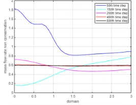
The above figure here we are plotting the mass flow rate againts the different time step.
2.
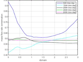
The above fogure its showing the variation of non conservation mass flow rate againt the diffrent time steps.
3.
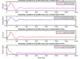
The above figure is showing the variation of density,time,velocity and mach number at throttle with respect the given time step.
4.
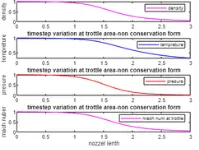
The above figure its shown that the varion of variables with respect to the nozzle length of non conservation form.
5.
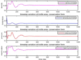
The above figure its shown that the variation of variables with respect to the nozzle length of the conservation form.
6.
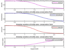
The above figure its shown that the variation of variables with respect to the nozzle length of the conservation form.
7.
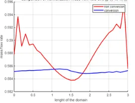
The above figure shows the mass flow rate comparison of conservation and non conservation form.