Project 2 - Rankine cycle Simulator
Introduction:-
The Rankine cycle is an idealized thermodynamic cycle describing the process by which certain heat engines, such as steam turbines or reciprocating steam engines, allow mechanical work to be extracted from a fluid as it moves between a heat source and heat sink.
Heat energy is supplied to the system via a boiler where the working fluid (typically water) is converted to a high pressure gaseous state (steam) in order to turn a turbine. After passing over the turbine the fluid is allowed to condense back into a liquid state as waste heat energy is rejected before being returned to boiler, completing the cycle. Friction losses throughout the system are often neglected for the purpose of simplifying calculations as such losses are usually much less significant than thermodynamic losses, especially in larger systems.
Program Code:-
clear all
close all
clc

% Information of all process

fprintf('Rankine Cycle Simulator\n');
fprintf('1-2 Isentropic Expansion in the Turbine\n');
fprintf('2-3 Constant Pressure heat Rejection by the Condenser\n')
fprintf('3-2 Isentropic Compression in the pump\n')
fprintf('4-1 Constant Pressure Heat Addition by the Boiler\n')

% Taking Input Arguments

P1 = input('Enter the pressure at the turbine Inlet (bar): ');
T1 = input('Enter the temperature at the turbine inlet (Degree Celsius): ');
P2 = input('Enter the pressure at the Condenser (bar): ');

fprintf(' Result\n');

% General properties Calculation

% Calculation of Cp value at P1 & P2 for saturated liquid & vapor

CP1_L = XSteam('CpL_p',P1);
CP1_V = XSteam('CpV_p',P1);
CP2_L = XSteam('CpL_p',P2);
CP2_V = XSteam('CpV_p',P2);

% Calculation of saturation temperature at P1 & P2

Tsat_P1 = XSteam('Tsat_p',P1);
Tsat_P2 = XSteam('Tsat_p',P2);

% Calculation of Enthalpy & Entropy at saturation points

% Calculation of saturation properties at state 1

Hg_1 = XSteam('hV_p',P1);
Sg_1 = XSteam('sV_p',P1);

% Calculation of saturation properties at state 2

Hg_2 = XSteam('hV_p',P2);
Sg_2 = XSteam('sV_p',P2);

% calculation of saturation properties at state 3

Hf_3 = XSteam('hL_p',P2);
Sf_3 = XSteam('sL_p',P2);

% calculation of saturation properties at state 4

Hf_4 = XSteam('hL_p',P1);
Sf_4 = XSteam('sL_p',P1);

% Calculation of process properties at state 1

fprintf('At State point 1 ');

fprintf(' P1 is : %f Bar ',P1);

fprintf(' T1 is : %f degC ',T1);

H1 = XSteam('h_pT',P1,T1);
fprintf(' H1 is : %f kJ/kg ',H1);

S1 = XSteam('s_pT',P1,T1);
fprintf(' S1 is : %f kJ/kg ',S1);

% Calculation of process properties at state 2

fprintf(' At state point 2 ');

fprintf(' P2 is : %f Bar ',P2);

S2 = S1;
fprintf(' S2 is : %f kJ/kgK ',S2);

% Calculating value of X

if(S2<=Sg_2)
    X2 = (S2 - Sf_3)/(Sg_2 - Sf_3); % Dryness fraction at state point 2
else
    X2 = 1;
end
fprintf(' X2 is : %f ',X2);

% Calculatinng value of T2

if(X2<1)
    T2 = Tsat_P2;
else
    %S2 = Sg_2 + CP2_V*(log(T2/Tsat_P2))
    T2 = (Tsat_P2+273.15)*exp((S2-Sg_2)/CP2_V);
    T2 = T2-273.15;
end
fprintf(' t2 is : %f degC ',T2)

if(X2<1)
    H2 = Hf_3 + X2*(Hf_3-Hg_2);
else
    H2 = XSteam('h_pT',P2,T2);
end
fprintf(' H2 is : %f kJ/kg ',H2)

% Calculation of process properties at state 3

fprintf(' At state point 3 ')

P3 = P2;
fprintf(' P3 is : %f bar ',P3)

V3 = XSteam('vL_p',P3);

T3 = Tsat_P2;     % No subcooling assumption
fprintf(' t3 is : %f degC ',T3)

H3 = Hf_3;
fprintf(' H3 is : %f kJ/kg ',H3)

S3 = Sf_3;
fprintf(' S3 is : %f kJ/kg ',S3)

% Calculation of process properties at state 4

fprintf(' At state point 4 ')

P4 = P1;
fprintf(' P4 is : %f bar ',P4)

S4 = S3;
fprintf(' S4 is : %f kJ/kgK ',S4)

Wp = V3*(P4-P3)*100;
H4 = Wp + H3;
fprintf(' H4 is : %f kJ/kg ',H4)

T4 = (Tsat_P1+273.15)/(exp((Sf_4-S4)/CP1_L));
T4 = T4-273.15;
fprintf(' T4 is : %f degC ',T4)

% Plotting saturation Liquid & vapor lines

temp = linspace(1, T1, 1000);
for i = 1: length(temp)
    H_L(i) = XSteam('hL_T',temp(i));
    H_V(i) = XSteam('hV_T',temp(i));
    S_L(i) = XSteam('sL_T',temp(i));
    S_V(i) = XSteam('sV_T',temp(i));
end

% Plotting T-S

figure(1)
hold on
plot([S1 S2], [T1 T2], 'r','linewidth',2)
text(S1,T1,'1')
text(S2,T2,'2')
plot([S2 Sg_2], [T2 Tsat_P2], 'r','linewidth',2)
text(Sg_2, Tsat_P2, '2s')
plot([Sg_2 S3],[Tsat_P2 T3],'r','lineWidth',2)
text(S3,T3,'3')
plot([S3 S4], [T3 T4],'r','linewidth',2)
text(S4,T4,'4')
plot([S4 Sf_4],[T4 Tsat_P1],'r','linewidth',2)
text(Sf_4,Tsat_P1,'4s')
plot([Sf_4 Sg_1],[Tsat_P1 Tsat_P1],'r','linewidth',2)
text(Sg_1,Tsat_P1,'1s')
plot([Sg_1 S1],[Tsat_P1 T1],'r','linewidth',2)
plot(S_L,temp,'b','linestyle','--','linewidth',1)
plot(S_V,temp,'b','linestyle','--','linewidth',1)
title('T-S Diagram of Ideal rankine Cycle')
xlabel('Specific Entropy (kJ/kgK)')
ylabel('Temperature (degC)')

% Plotting H-S

figure(2)
hold on
plot([S1 S2],[H1 H2],'r','linewidth',2)
text(S1,H1,'1')
text(S2,H2,'2')
plot([S2 Sg_2],[H2 Hg_2],'r','linewidth',2)
text(Sg_2,Hg_2,'2s')
plot([Sg_2 S3],[Hg_2 H3],'r','linewidth',2)
text(S3,H3,'3')
plot([S3 S4],[H3 H4],'r','linewidth',2)
text(S4,H4,'4')
plot([S4 Sf_4],[H4 Hf_4],'r','linewidth',2)
text(Sf_4,Hf_4,'4s')
plot([Sf_4 Sg_1], [Hf_4 Hg_1],'r','linewidth',2)
text(Sg_1,Hg_1,'1s')
plot([Sg_1 S1],[Hg_1 H1],'r','linewidth',2)
plot(S_L,H_L,'b','linestyle','--','linewidth',1.5)
plot(S_V,H_V,'b','linestyle','--','linewidth',1.5)
title('H-S Diagram of Ideal rankine Cycle')
xlabel('Specific Entropy (kJ/kgK)')
ylabel('Specific Enthalpy (kJ/kg)')

% Calculation of work done,ssc & efficiency

Wt = H1-H2;
fprintf(' Work by turbine is : %f kJ/kg ',Wt)
fprintf(' Work by compressor is : %f kJ/kg ',Wp)
Wnet = Wt-Wp;
fprintf(' Net Work done is : %f kJ/kg ',Wnet)
Qin = H1-H4;
eff_thermal = Wnet*100/Qin;      % Efficiency
fprintf(' Thermal efficiency is : %f ',eff_thermal);
disp('%')
SSC = 3600/Wt;                   % Specific steam consumption
fprintf(' S.S.C is : %f kg/kWh ',SSC)
Output:-
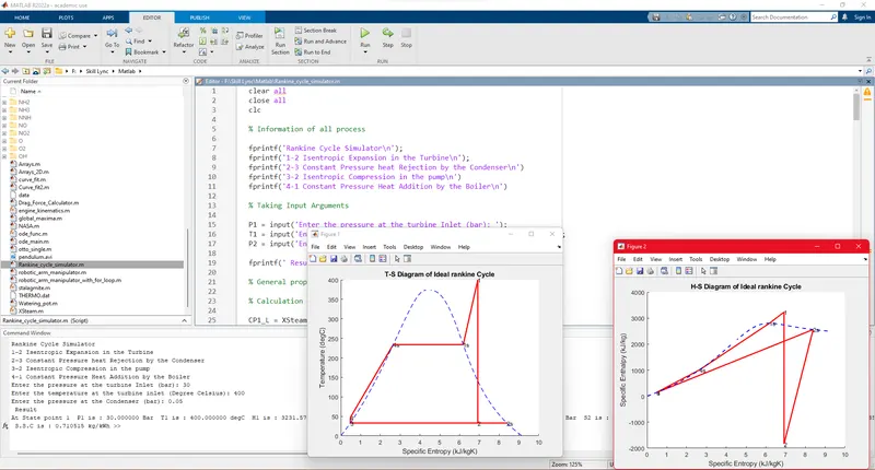
Explanation:-
For this program we are using steam table XSteam.m
Used clear all, close all, clc
Description of all process
Take input parameters
Calculation :-
Saturation Temp at P1 & P2
Saturation properties at state 1,2,3 & 4
Process properties at state 1,2,3 & 4
Plotting Saturation liquid & vapor lines
T-S plot
H-S plot
Work done, heat, SSC & Efficiency.