Week 7 - Simulation of a 1D Super-sonic nozzle flow simulation using Macormack Method
AIM
to simulate the isentropic flow through a quasi 1D subsonic-supersonic nozzle. derive both the conservation and non-conservation forms of the governing equations and sovle them using the MacCormack's technique. to determine the steady-state temperature distribution for the flow-field variables and investigate the difference between the two forms of governing equations by comparing their solutions.
OBJECTIVE
need to show the following plots inside your report
1. Steady-state distribution of primitive variables inside the nozzle
2. Time-wise variation of the primitive variables
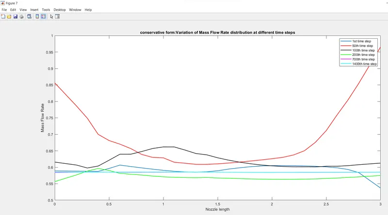
3. Variation of Mass flow rate distribution inside the nozzle at different time steps during the time-marching process
4. Comparison of Normalized mass flow rate distributions of both forms
EXPLANATION
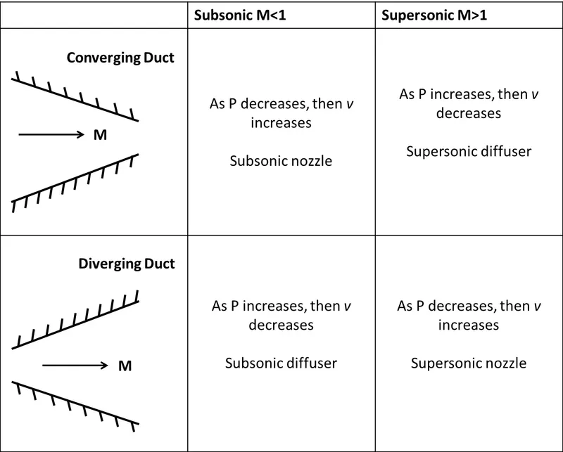
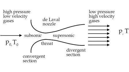
A de Laval nozzle (or convergent-divergent nozzle) features a length of tube pinched in the middle (the throat). At subsonic velocities a converging tube causes the gas flow to accelerate. At supersonic velocities, however, the tube must be divergent in order for the gas to expand and accelerate. Among many applications of the de Laval nozzle are rocket propulsion and supersonic jet engines.
ASSUMPTIONS
- flow properties vary w.r.t X-Axis only.THerefore ,it is a quasi 1D flow
- steady,isentropic flow through convergent-divergent nozzle
STEPS TO BE FOLLOWED
- the governing equations are modified for simplification in soving the equations
- These equations which are in the form of PDEs are suitable for time marching solution of 1D Qausi flow
- these equations are then expressed in the FDM form i.e.grid points(nodes)are assigned to equations and presented in forward differencing
- since these values are only 1st order accurate,corrector step is used to make it 2nd order accurate
- then a mean value is taken of these value which is considered as final value
- boundary and initial conditions are assigned
1.GOVERNING EQUATIONS
NON-CONSERVATIVE
continuity equation
`(delrho')/(delt)=-rho'*(delv')/(delx')-rho'*v'*(dellnA')/(delx')-v'*(delrho')/(delx')`
momentum equation
`(delv')/(delt')=-v'*(delv')/(delx')-1/gamma*((delT')/(delx')+(T')/(rho')*(delrho')/(delx'))`
energy equation
`(delT')/(delt')=-v*(delT')/(delx')-(gamma-1)*T'*[(delv')/(delx')+v'*(del(lnA))/(delx')]`
CONSERVATIVE
continuity equation
`(del(rho'A'))/(delt)+(del(v'rho'A'))/(delx')=0`
momentum equation
`(del(rho'A'v'))/(delt')+(del[rho'A'v'^2+1/gamma*p'A'])/(delx')=1/gamma*p'*(delA')/(delx')`
energy equation
`(del[rho'*((e')/(gamma-1)+gamma/2*v'^2)A'])/(delt')+(del[rho'*((e')/(gamma-1)+gamma/2*v'^2)*v'A'+p'A'v'])/(delx')=0`
2.FDM USING MACROMACK METHOD (EXPLICIT) FOR NUMERICAL SOLUTION
- The nozzle is divide into nodes along x-axis (along the flow).mesh size is given by dx`/Deltax`.these nodes are evenly distributed and spaced
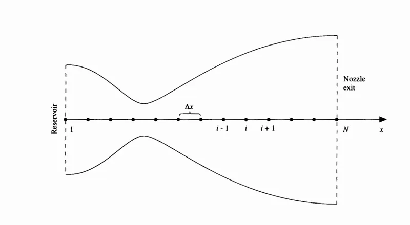
- the 1st node labeled as 1 in the above figure is assumed to be the reservoir
- here point i is any point on the axis,with i+1 as forward piont and i-1 as backward point adjacent to i
all numerical models developed from equation in the conservative form and used FVM are consistent. Therefore, an explicit numerical method that used discretized equations in the conservative form by FVM will be consistent. However, the numerical method stability will be given by CFL (Courant-Friedrichs-Lewy) condition, where the CFL condition depend on time step, grid size, among others information. So, an explicit numerical method is called "Conditionally stable".
methods to solve the governing equations of fluid flow, such as:
Euler Method, Lax-Wendroff Method, Brailovskaya Method, Range-Kutta Method, MacCormack Method, etc. When is made a comparison among these method some have advantages and disadvantages in some features.
The MacCormack Method has some important features and is large applied to solve compressible fluid flow problems.
The MacCormack is a variation of two steps Lax-Wendroff Method, but, more efficient to solve PDEs non-liners, generating good solutions to discontinuities of this equations.
the MacCormack Method is a two steps method, this is, it calculates a "Predictor Step" and followed it calculates a "Corrector Step", defining the final value from an arithmetic mean. If predictor step used a forward differential operator and corrector step use backward differential operator. The method must follow this scheme to ensure the main feature a second-order of accuracy for time and space.
flow properties vary w.r.t time t,
NON-CONSERVATIVE FORM
Predictor step ,spatial derivatives as forward differencing
Continuity Equation:-

Momentum Equation:-

Energy Equation

From the above equations, the predicted value of `rho`,v,T can be calculated
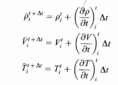
But these values are only 1st order accurate,so corrector step is needed for to make it 2nd order accurate
In the corrector step ,the predicted values are substitued in the formula
Continuity Equation
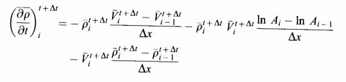
Momentum Equation

Energy Equation
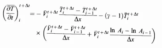
using the above equations,the average time derivative is formulated
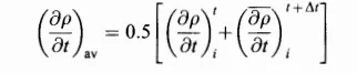
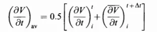
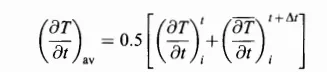
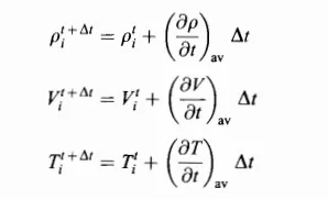
corrected values
CONSERVATION FORM
define the solutions vectors
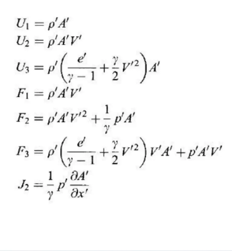
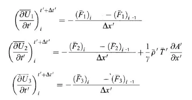
finding source vectors with the help of initial condition , then with the help of source vector we hav eto find flux vectors
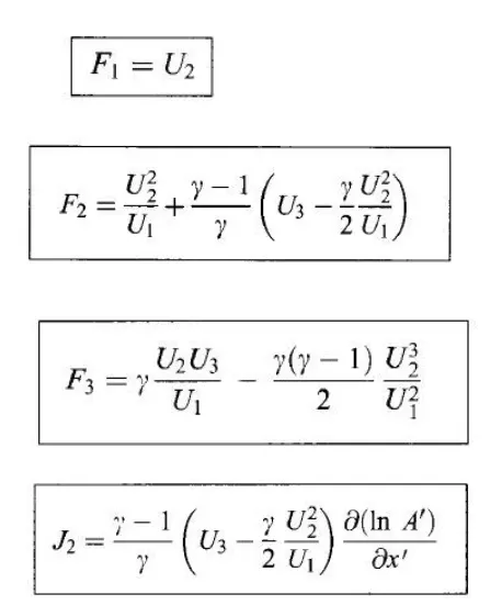
Predictor step,spatial derivatives as forward differencing
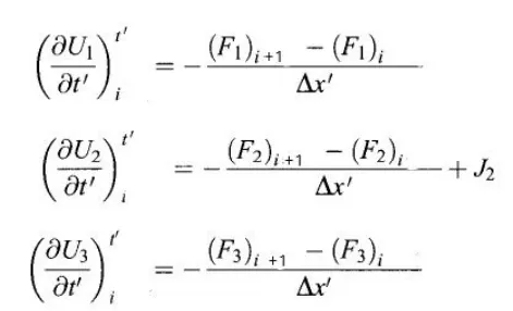
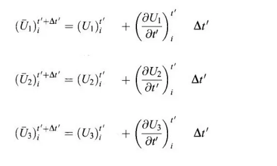
finding the predicted values of U1,U2,U3
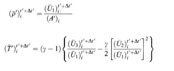
using these values,finding predicted values of primitive variables
corrector step
But these values are only 1st order accurate,so corrector step is needed for to make it 2nd order accurate
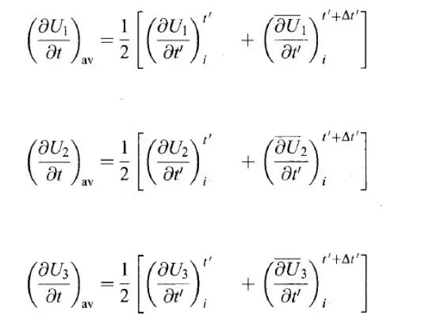
average time derivatives
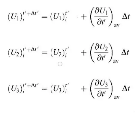
final corrected values of U1,U2,U3
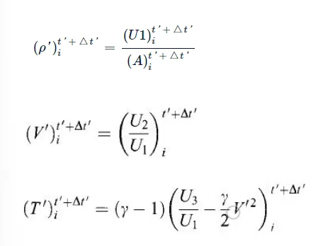
Obataining the values of primitive variable with the help of U1,U2,U3
Calculation of TimeStep size
`Deltat=C*(Deltax)/(a+v)`
where,
C=courant number=0.5
a=speed of sound
v=velocity
BOUNDARY AND INITIAL CONDITIONS
NON-CONSERVATIVE
Nozzle area

Initial conditions
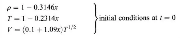
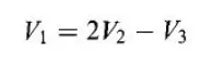
Boundary condition at Inlet
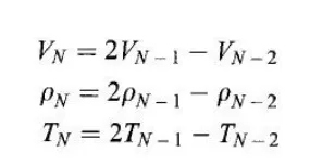
Boundary condition at Outlet
CONSERVATIVE FORM
Nozzle area

Initial conditions
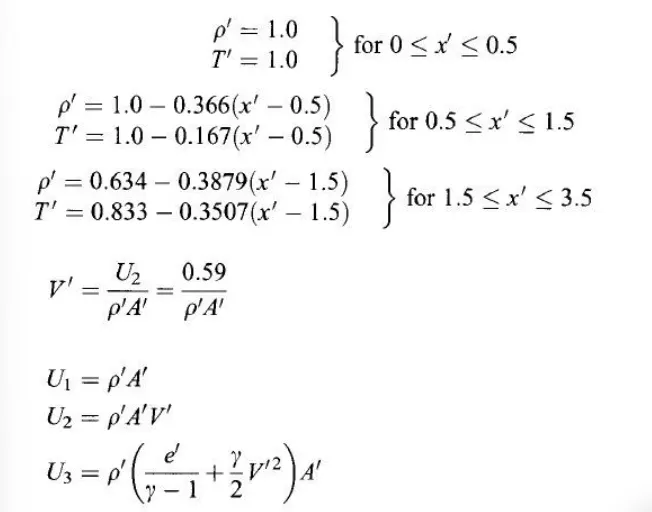
Boundary condition at Inlet
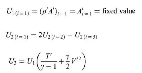
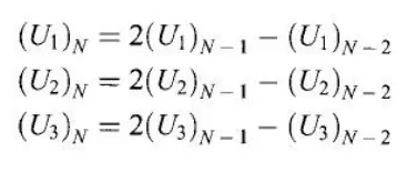
Boundary condition at Outlet
CODE
MAIN CODE
clear all
close all
clc

%input
n=31;
nt=1400;
x=linspace(0,3,31);
dx=3/(n-1);

%Non conservative form
[rho,v,t,P,M,rho_t,v_t,t_t,P_t,M_t,m]=non_conservative(n,nt,x,dx);

%conservative form
[rho_c,v_c,t_c,P_c,M_c,rho_t_c,v_t_c,t_t_c,P_t_c,M_t_c,m_c,dt]=conservative(n,nt,x,dx);

%plots for non conservative ,mach number , pressureand temperature VS
%distanceat 1400 timestep
figure(1)
subplot(4,1,1)
plot(x,M,'r','linewidth',1.1)
title('Non-conservative form :Distribution primitive variables along the nozzle length')
xlabel('Nozzle length')
ylabel('Mach Number')

subplot(4,1,2)
plot(x,P,'m','linewidth',1.1)
xlabel('Nozzle length')
ylabel('Pressure')

subplot(4,1,3)
plot(x,rho,'g','linewidth',1.1)
xlabel('Nozzle length')
ylabel('Density')

subplot(4,1,4)
plot(x,t,'linewidth',1.1)
xlabel('Nozzle length')
ylabel('Temperature')

%%plots for  conservative ,mach number , pressureand temperature VS
%distance at 1400 timestep
figure(2)
subplot(4,1,1)
plot(x,M_c,'r','linewidth',1.1)
title('conservative form :Distribution primitive variables along the nozzle length')
xlabel('Nozzle length')
ylabel('Mach number')

subplot(4,1,2)
plot(x,P_c,'m','linewidth',1.1)
xlabel('Nozzle length')
ylabel('Pressure')

subplot(4,1,3)
plot(x,rho_c,'g','linewidth',1.1)
xlabel('Nozzle length')
ylabel('density ')
subplot(4,1,4)
plot(x,t_c,'linewidth',1.1)
xlabel('Nozzle length')
ylabel(' temperature')

%plots for Non conservative ,mach number , pressureand temperature VS
%distance at thoart area

figure(3)
subplot(4,1,1)
plot(M_t,'g','linewidth',1.1)
title('conservative form :Distribution primitive variables at thoart with varying timesteps')
ylabel('Mach Number')

subplot(4,1,2)
plot(P_t,'r','linewidth',1.1)
ylabel('Pressure')

subplot(4,1,3)
plot(rho_t,'linewidth',1.1)
ylabel('Density')

subplot(4,1,4)
plot(t_t,'m','linewidth',1.1)
ylabel('Temperature')

%plots for  conservative ,mach number , pressureand temperature VS
%distance at thoart area

figure(4)
subplot(4,1,1)
plot(M_t_c,'g','linewidth',1.1)
title('conservative form :Distribution primitive variables at thoart with varying timesteps')
ylabel('Mach Number')

subplot(4,1,2)
plot(P_t_c,'r','linewidth',1.1)
ylabel('Pressure')

subplot(4,1,3)
plot(rho_t_c,'linewidth',1.1)
ylabel('Density')

subplot(4,1,4)
plot(t_t_c,'m','linewidth',1.1)
ylabel('Temperature')

%Mass flow rate distribution inside the nozzle

figure(5)
plot(x,m,'m','linewidth',1.1)
hold on
plot(x,m_c,'linewidth',1.1)
title('Comparisons of normalized mass flow rate distributions of both forms')
xlabel('Nozzle length')
ylabel('Mass Flow Rate')
legend('Non Conservative Form','Conservative Form')


figure(6)
legend('1st time step','50th time step','100th time step','200th time step','700th time step','1400th time step')
title('Non-conservative form:Variation of Mass Flow Rate distribution at different time steps')
xlabel('Nozzle length')
ylabel('Mass Flow Rate')


figure(7)
legend('1st time step','50th time step','100th time step','200th time step','700th time step','1400th time step')
title('conservative form:Variation of Mass Flow Rate distribution at different time steps')
xlabel('Nozzle length')
ylabel('Mass Flow Rate')
FUNCTION FOR NON-CONSERVATIVE FORM
function[rho,v,t,P,M,rho_t,v_t,t_t,P_t,M_t,m]=non_conservative(n,nt,x,dx)

%initial profiles
rho=1-0.3146*x;
t=1-0.2314*x;
v=(0.1+1.09*x).*(t).^0.5;

gamma=1.4;

%area
a=1+2.2*(x-1.5).^2;

dt=min(0.5*dx./(v+sqrt(t)));

%outer time step
for k=1:nt

    %copy of previous values of variables
    rho_old=rho;
    v_old=v;
    t_old=t;

    %predictor method
    for j=2:n-1
        dvdx=(v(j+1)-v(j))/dx;
        drhodx=(rho(j+1)-rho(j))/dx;
        dtdx=(t(j+1)-t(j))/dx;
        dlogadx=(log(a(j+1))-log(a(j)))/dx;

        %contuinity equation
        drhodt_p(j)=-rho(j)*dvdx-rho(j)*v(j)*dlogadx-v(j)*drhodx;

        %momentum equation
        dvdt_p(j)=-v(j)*dvdx-(1/gamma)*(dtdx+(t(j)/rho(j))*drhodx);

        %energy equation(here dtdt means time derivative)
        dtdt_p(j)=-v(j)*dtdx-(gamma-1)*t(j)*((dvdx+v(j)*dlogadx));

        %creating a copy of new values
        rho(j)=rho(j)+drhodt_p(j)*dt;
        v(j)=v(j)+dvdt_p(j)*dt;
        t(j)=t(j)+dtdt_p(j)*dt;
    end

    %Corrector method
    for j=2:n-1
        dvdx=(v(j)-v(j-1))/dx;
        drhodx=(rho(j)-rho(j-1))/dx;
        dtdx=(t(j)-t(j-1))/dx;
        dlogadx=(log(a(j))-log(a(j-1)))/dx;

        %contuinity equation
        drhodt_c(j)=-rho(j)*dvdx-rho(j)*v(j)*dlogadx-v(j)*drhodx;

        %momentum equation
        dvdt_c(j)=-v(j)*dvdx-(1/gamma)*(dtdx+(t(j)/rho(j))*drhodx);

        %energy equation(here dtdt means time derivative)
        dtdt_c(j)=-v(j)*dtdx-(gamma-1)*t(j)*((dvdx+v(j)*dlogadx));

    end
    %Average time derivative
    drhodt=0.5*(drhodt_p+drhodt_c);
    dvdt=0.5*(dvdt_p+dvdt_c);
    dtdt=0.5*(dtdt_p+dtdt_c);

    %final solution update
    for i=2:n-1
        rho(i)=rho_old(i)+drhodt(i)*dt;
        v(i)=v_old(i)+dvdt(i)*dt;
        t(i)=t_old(i)+dtdt(i)*dt;
    end

    %boundary condition
    %inlet
    v(1)=2*v(2)-v(3);

    %outlet
    v(n)=2*v(n-1)-v(n-2);
    rho(n)=2*rho(n-1)-rho(n-2);
    t(n)=2*t(n-1)-t(n-2);

    %calculation of presseure mach number and mass flow rate
    P=rho.*t;
    M=v./sqrt(t);
    m=rho.*a.*v;

    %calculation of presseure mach number and mass flow rate at thoart
    P_t(k)=P(16);
    v_t(k)=v(16);
    M_t(k)=M(16);
    t_t(k)=t(16);
    rho_t(k)=rho(16);

    %variation of mass flow rate distribution inside the nozzle at
    %different time steps
    figure(6)
    if k==1
        plot(x,m,'linewidth',1.3)
        hold on
    elseif k==50
        plot(x,m,'r','linewidth',1.3)
        hold on
    elseif k==100
        plot(x,m,'k','linewidth',1.3)
        hold on
    elseif k==200
        plot(x,m,'g','linewidth',1.3)
        hold on
    elseif k==700
        plot(x,m,'m','linewidth',1.3)
        hold on
    elseif k==1400
        plot(x,m,'cyan','linewidth',1.3)
        hold on
    end
end
end
FUNCTION FOR CONSERVATIVE FORM
function [rho_c,v_c,t_c,P_c,M_c,rho_t_c,v_t_c,t_t_c,P_t_c,M_t_c,m_c,dt]=conservative(n,nt,x,dx)

%Initial Profiles
for i=1:n
    if (0<=x(i) && x(i)<=0.5)
        rho_c(i)=1;
        t_c(i)=1;
    elseif (0.5<=x(i) && x(i)<=1.5)
        rho_c(i)=1-0.366*(x(i)-0.5);
        t_c(i)=1-0.167*(x(i)-0.5);
    elseif (1.5<=x(i) && x(i)<=3.5)
        rho_c(i)=0.634-0.3879*(x(i)-1.5);
        t_c(i)=0.833-0.3507*(x(i)-1.5);
    end
end

%area
a=1+2.2*(x-1.5).^2;
gamma=1.4;

v_c=0.59./(rho_c.*a);

%solutions vectors
u1=rho_c.*a;
u2=rho_c.*a.*v_c;
u3=rho_c.*(t_c/(gamma-1)+(gamma/2)*v_c.^2).*a;
dt=min(0.5*(dx./(v_c+sqrt(t_c))));

%outer time step
for k=1:nt
    %copy of values of u1,u2,u3
    u1_old=u1;
    u2_old=u2;
    u3_old=u3;

    %Flux vectors
    f1=u2;
    f2=(u2).^2./u1+((gamma-1)/gamma)*(u3-(gamma/2)*((u2).^2./u1));
    f3=(gamma*u2.*u3)./u1-(gamma*(gamma-1))/2*((u2).^3./(u1).^2);

    %predictor method
    for j=2:n-1
        J2=(1/gamma)*rho_c(j)*t_c(j)*((a(j+1)-a(j))/dx);

        %contuinity equation
        du1dt_p(j)=-(f1(j+1)-f1(j))/dx;

        %momentum equation
        du2dt_p(j)=(-(f2(j+1)-f2(j))/dx)+J2;

        %energy equation
        du3dt_p(j)=-(f3(j+1)-f3(j))/dx;

        %solution update
        u1(j)=u1(j)+du1dt_p(j)*dt;
        u2(j)=u2(j)+du2dt_p(j)*dt;
        u3(j)=u3(j)+du3dt_p(j)*dt;
    end
    %updating primitive variables
    rho_c=u1./a;
    t_c=(gamma-1)*((u3)./(u1)-(gamma/2)*((u2)./(u1)).^2);

    %updating flux vectors
    f1=u2;
    f2=(u2).^2./u1+((gamma-1)/gamma)*(u3-(gamma/2)*((u2).^2./u1));
    f3=(gamma*u2.*u3)./u1-(gamma*(gamma-1))/2*((u2).^3./(u1).^2);

    %corrector method
    for j=2:n-1
        J2=(1/gamma)*rho_c(j)*t_c(j)*((a(j)-a(j-1))/dx);

        %contuinity equation

        %contuinity equation
        du1dt_c(j)=-(f1(j)-f1(j-1))/dx;

        %momentum equation
        du2dt_c(j)=(-(f2(j)-f2(j-1))/dx)+J2;

        %energy equation
        du3dt_c(j)=-(f3(j)-f3(j-1))/dx;


    end
    %average time derivative
    du1dt=0.5*(du1dt_c+du1dt_p);
    du2dt=0.5*(du2dt_c+du2dt_p);
    du3dt=0.5*(du3dt_c+du3dt_p);

    %final solution update
    for m=2:n-1
        u1(m)=u1_old(m)+du1dt(m)*dt;
        u2(m)=u2_old(m)+du2dt(m)*dt;
        u3(m)=u3_old(m)+du3dt(m)*dt;
    end

    %boundary conditions
    %inlet
    u1(1)=a(1);
    u2(1)=2*u2(2)-u2(3);
    u3(1)=u1(1)*(t_c(1)/(gamma-1)+(gamma/2)*v_c(1)^2);

    %outlet
    u1(n)=2*u1(n-1)-u1(n-2);
    u2(n)=2*u2(n-1)-u2(n-2);
    u3(n)=2*u3(n-1)-u3(n-2);

    %Final uadate of primitive variables
    rho_c=u1./a;
    t_c=(gamma-1)*((u3)./(u1)-(gamma/2)*((u2)./(u1)).^2);
    v_c=(u2)./(u1);

    %Calculation of pressure, Mach Number and mass flow rate
    P_c=rho_c.*t_c;
    M_c=v_c./sqrt(t_c);
    m_c=rho_c.*a.*v_c;

    %calculation of pressure, Mach Number and Mass folw rate at thoart
    P_t_c(k)=P_c(16);
    v_t_c(k)=v_c(16);
    M_t_c(k)=M_c(16);
    t_t_c(k)=t_c(16);
    rho_t_c(k)=rho_c(16);

    %variation of mass flow rate distribution inside the nozzle at
    %different time steps
    figure(7)
    if k==1
        plot(x,m_c,'linewidth',1.3)
        hold on
    elseif k==50
        plot(x,m_c,'r','linewidth',1.3)
        hold on
    elseif k==100
        plot(x,m_c,'k','linewidth',1.3)
        hold on
    elseif k==200
        plot(x,m_c,'g','linewidth',1.3)
        hold on
    elseif k==700
        plot(x,m_c,'m','linewidth',1.3)
        hold on
    elseif k==1400
        plot(x,m_c,'cyan','linewidth',1.3)
        hold on
    end
end
end
CODE EXPLANATION
MAIN CODE
- Input values like number of nodes(grid points),number of timesteps (nt),length of nozzle/fluid domain (x),distance between nodes/mesh size(dx) are assigned.
- conservative.m and non_conservative.m functions are being called in the main code and parameters like density(rho),temperature(T),Mach number(M),velocity(v) as matrix or as separate value in Thorat region is calculated and being called in main code
- Plot graphs for conservative and non-conservative form by variation in parameter (density,temperature,Mach Number,velocity) along the length of nozzle
- Plot graphs for conservative and non-conservative form by variation in parameter (density,temperature,Mach number,velocity) at Thorat with timesteps
- Plot graphs for conservative and non-conservative form by variation in mass flow rate at different timesteps
- comparing the mass flow rates of conservative and non-conservative form .
FUNCTION CODE FOR NON-CONSERVATIVE FORM
- input values of number of nodes(n),number of timesteps(nt),range of nozzle length (x),mesh size(dx).
- initial profiles of density,temperature and velocity are assigned
- for calculating the speed of sound `v=sqrt(gammaRt)`,gamma value is assigned
- For calculating the area at different values of x ,a variable 'a' is assigned having relation with x
- Calculating dt with the formula
- creating a outer loop for time step from 1 to nt,to calculate variables at different values of timesteps
- creating a copy previous variables and assigning them a new variable like rho_old,v_old,t_old for density,velocity, temperature respectively.
- creating a loop for predictor method from 2 to n-1,(to calculate the values from all nose except the 1st and last,as they are boundary conditions,),to calculate the value of density, temperature,velocity at each node
- Differentiating velocity,density,temperature and log(area) w.r.t x in forward differencing scheme as these values are required in continuity,momentum,energy equation in predictor method
- calculating continuity(drhodt_p),momentum(dvdt_p),energy (dtdt_p)equations
- creating a matrix copy of new values by adding the previous value rho,v,tand drhodt_p,dvdt_p,dtdt_p respectively.
- end of the predictor loop
- creating a loop for corrector method from 2 to n-1,(to calculate the values from all nose except the 1st and last,as they are boundary conditions,),to calculate the value of density, temperature,velocity at each node
- Differentiating velocity,density,temperature and log(area) w.r.t x in rearward differencing scheme as these values are required in continuity,momentum,energy equation in predictor method
- calculating continuity(drhodt_c),momentum(dvdt_c),energy (dtdt_c)equations
- end of corrector loop
- calculating average time derivatie by adding the values of density,velocity,temperature of both predictor and corrector method
- updating final solution by adding the old values rho_old,v_old,t_old and drhodt*dt,dvdt*dt,dtdt*dt respectively for every node from2 to n-1.
- assigning the boundary and initial values
- calculating pressure, density and mach number as matix and in thoart region
- plotting a graph for different value of timesteps
FUNCTION CODE FOR CONSERVATIVE FORM
- input values of number of nodes(n),number of timesteps(nt),range of nozzle length (x),mesh size(dx).
- initial profiles of density,temperature and velocity are assigned
- for calculating the speed of sound `v=sqrt(gammaRt)`,gamma value is assigned
- For calculating the area at different values of x ,a variable 'a' is assigned having relation with x
- Calculating dt with the formula
- defining u1,u2,u3
- creating a outer loop for time step from 1 to nt,to calculate variables at different values of timesteps
- creating a copy previous variables(solution vectors)
- defining flux vectors
- creating a loop for predictor method from 2 to n-1,(to calculate the values for all node except the 1st and last,as they are boundary conditions,),to calculate the value of solution vector at each node
- Differentiating solution vectors w.r.t x in forward differencing scheme as these values are required in continuity,momentum,energy equation in predictor method
- calculating continuity(du1dt_p),momentum(du2dt_p),energy (du3dt_p)equations
- creating a matrix copy of new values by adding the previous value u1,u2,u3 and du1dt_p,du2dt_p,du3dt_p respectively.
- end of the predictor loop
- updating velocity and temperature matrix
- updating flux vectors
- creating a loop for corrector method from 2 to n-1,(to calculate the values from all nose except the 1st and last,as they are boundary conditions,),to calculate the value of solution vectors at each node
- Differentiating velocity,density,temperature and log(area) w.r.t x in rearward differencing scheme as these values are required in continuity,momentum,energy equation in predictor method
- calculating continuity(du1dt_c),momentum(du2dt_c),energy (du3dt_p)equations
- end of corrector loop
- calculating average time derivatie by adding the values of solution vectors of both predictor and corrector method
- updating final solution by adding the old values u1_old,u2_old,u3_old and du1dt*dt,du2dt*dt,du3dt*dt respectively for every node from2 to n-1.
- assigning the boundary and initial values
- calculating pressure, density,temperature,velocity and mach number as matix and in thoart region
- plotting a graph for different value of timesteps
OUTPUT & RESULT
FIGURE 1
temperature,density and pressure decreses as length of nozzle increases.
but mach number increases as length of nozzle increases
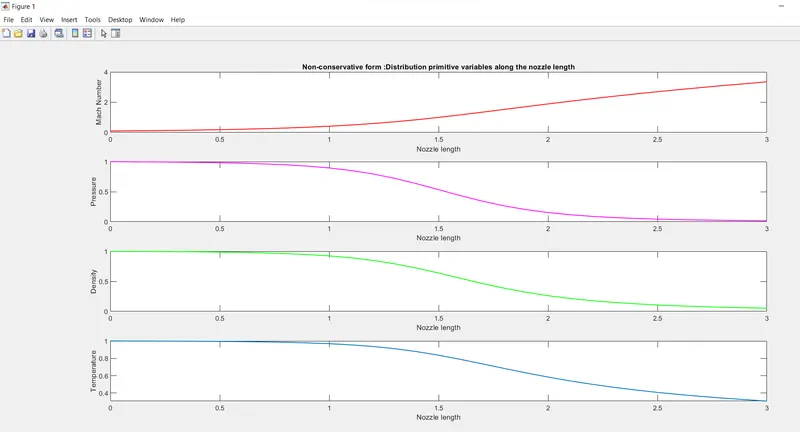
FIGURE 2
temperature,density and pressure decreses as length of nozzle increases.
but mach number increases as length of nozzle increases
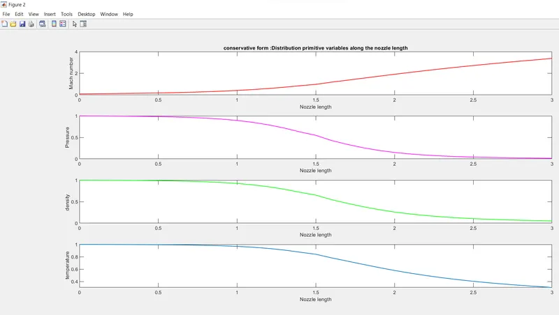
FIGURE 3
some fluctuations in all primitive variables initially but later plots become linear ,implying a steady state
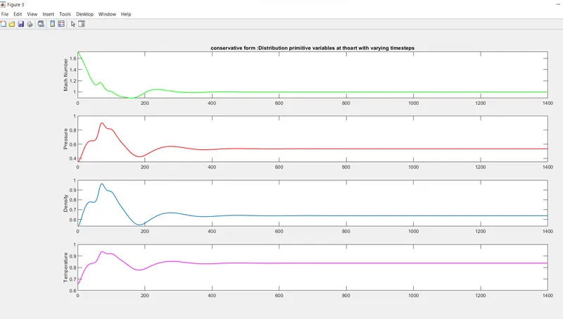
FIGURE 4
some fluctuations in all primitive variables initially but later plots become linear ,implying a steady state
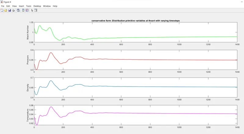
FIGURE 5
conservative form yields a better mass flow distribution than non-conservative form
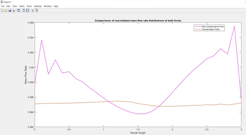
FIGURE 6
as the number of timestep increases,solution reaches steady state
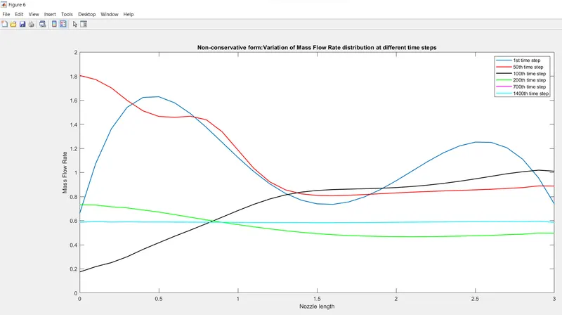
FIGURE 7
as the number of timestep increases(as seen in 700th&1400th),solution reaches steady state