Week 5.1 - Mid term project - Solving the steady and unsteady 2D heat conduction problem
AIM
Solve the 2D heat conduction equation by using the point iterative techniques that were taught in the class. The Boundary conditions for the problem are as follows;
Top Boundary = 600 K
Bottom Boundary = 900 K
Left Boundary = 400 K
Right Boundary = 800 K
To implement the following methods for solving implicit equations.
1. Jacobi
2. Gauss-seidel
3. Successive over-relaxation
absolute error criteria is 1e-4
OBJECTIVE
Write code for both implicit and explicit schemes (This is for the Transient Analysis only)
THEORY
Length og domain=1m
`(delT)/(delt)-alpha*((del^2T)/(delx^2)+(del^2T)/(dely^2)+(del^2T)/(delz^2))=0`heat conduction equation in 3D
the problem statement deals with 2D system
`(delT)/(delt)-alpha*((del^2T)/(delx^2)+(del^2T)/(dely^2))=0` .........(1)
steady state
in steady state,temperature w.r.t to time does not change i.e.`(delT)/(delt)=0`
therefore equation(1) changes to
`(del^2T)/(delx^2)+(del^2T)/(dely^2)=0`
`(del^2T)/(delx^2)+(del^2T)/(dely^2)=0`
expanding the terms using central differencing scheme
`(del^2T)/(delx)^2=(T(i-1,j)-2T(i,j)+T(i+1,j))/(Deltax)^2`
and
`(del^2T)/(dely)^2=(T(i,j-1)-2T(i,j)+T(i,j+1))/(Deltay)^2`
SOR facor,`omega =1.25`
1.JACOBI
`T(i,j)=(Told(i-1,j)+Told(i+1,j))/(k*(Deltax)^2)+(Told(i,j-1)+Told(i,j+1))/(k*(Deltay)^2)`
where `k=2*((Deltax)^2*(Deltay)^2)/((Deltax)^2+(Deltay)^2)`
2.GAUSS SEIDEL
`T(i,j)=(Told(i-1,j)+T(i+1,j))/(k*(Deltax)^2)+(Told(i,j-1)+T(i,j+1))/(k*(Deltay)^2)`
where `k=2*((Deltax)^2*(Deltay)^2)/((Deltax)^2+(Deltay)^2)`
3.SOR(SUCCESSIVE OVER REXALATION)
`T(i,j)=(1-omega)*Told(i,j)+omega*(Told(i-1,j)+T(i+1,j))/(k*(Deltax)^2)+(Told(i,j-1)+T(i,j+1))/(k*(Deltay)^2)`
where `k=2*((Deltax)^2*(Deltay)^2)/((Deltax)^2+(Deltay)^2)`
transient state
`(delT)/(delt)-alpha*((del^2T)/(delx^2)+(del^2T)/(dely^2))=0`
`(delT)/(delt)=alpha*((del^2T)/(delx^2)+(del^2T)/(dely^2))`
`(del^2T)/(delx)^2=(T(i-1,j)-2T(i,j)+T(i+1,j))/(Deltax)^2`
and
`(del^2T)/(dely)^2=(T(i,j-1)-2T(i,j)+T(i,j+1))/(Deltay)^2`
1.EXPLICIT TECHNIQUE
`T ( i , j )^ n = ( 1 − 2 k 1 − 2 k 2 ) ⋅ T ( i , j ) ^(n − 1) + k 1 ⋅ ( T ( i − 1 , j ) + T ( i +1, j ) ) ^(n − 1 )+ k 2 ⋅ ( T ( i , j − 1 ) + T ( i . j + 1 ) ) ^(n − 1)`
where`k1=alpha*(d^2t)/dx^2`
`k2=alpha*(d^2t)/dy^2`
2.IMPLICIT TECHNIQUE
JACOBI
`term1=1/(1+2*k1+2*k2)`
`term2=k1*term1`
`term3=k1*term1`
`T ( i , j )^ n = term1 ⋅ T ( i , j ) ^(n − 1) + term2⋅ ( T ( i − 1 , j ) + T ( i +1, j ) ) ^(old)+ term3⋅ ( T ( i , j − 1 ) + T ( i . j + 1 ) ) ^(old)`
GAUSS SEIDEL
`term1=1/(1+2*k1+2*k2)`
`term2=k1*term1`
`term3=k1*term1`
`T ( i , j )^ n = term1 ⋅ T ( i , j ) ^(n − 1) + term2⋅ ( T ( i − 1 , j ) + T ( i +1, j )^(old) ) + term3⋅ ( T ( i , j − 1 ) + T ( i . j + 1 )^(old) )`
SOR(SUCCESSIVE OVER REXALATION)
`term1=1/(1+2*k1+2*k2)`
-
`term2=k1*term1`
`term3=k1*term1`
`T ( i , j )^ n =(1-omega)T(i,j)^(old)+omega*( term1 ⋅ T ( i , j ) ^(n − 1) + term2⋅ ( T ( i − 1 , j ) + T ( i +1, j )^(old) ) + term3⋅ ( T ( i , j − 1 ) + T ( i . j + 1 )^(old) ))`
CODE
CODE FOR STEADY STATE USING IMPLICIT TECHNIQUE
clear all
close all
clc


%2D heat conduction at steady state using implicit technique
%inputs
L=1%length of domain
omega=1.25;%sor factor
nx=100;%grid size
ny=nx;
x=linspace(0,L,nx);
dx=x(2)-x(1);
y=linspace(0,L,ny);
dy=y(2)-y(1);
%Temperature matrix
T=300*ones(nx,ny);
%boundary condition given in problem statement
%T_left=400
%T_right=800
%T_bottom=900
%T_top=600
T(:,1)=400;
T(1,:)=900;
T(:,end)=800;
T(end,:)=600;
%edge refinement
T(1,1)=(900+400)/2;
T(1,end)=(900+800)/2;
T(end,1)=(400+600)/2;
T(end,end)=(800+600)/2;

Told=T;
k1=2*(dx^2+dy^2)/(dx^2*dy^2);

tol=1e-4;

error=9e9;

solver=input('Enter the number for the solver method: n Jacobi=1 n Gauss Seidel=2 n SOR=3 N Solver Type: ')
if solver==1
    tic
    jacobi_iter=1;
    %convergence loop
    while(error>tol)
        %nodal loop
        for j=2:ny-1
            for i=2:nx-1
                H=((Told(i-1,j)+Told(i+1,j))/(k1*dx^2));
                V=((Told(i,j-1)+Told(i,j+1))/(k1*dy^2));
                T(i,j)=H+V;
            end
        end
        error=max(max(abs(Told-T)));
        %updating old values
        Told=T;
        jacobi_iter=jacobi_iter+1;
        timecounter=toc;
        %creating a plot
        figure(1)
        [C,h]=contourf(x,y,T,'ShowText','on');
        colorbar
        colormap(jet)
        xlabel('xx')
        ylabel('yy')
        clabel(C,h)
        title(sprintf('2D steady state heat conduction  n Method:Jacobi n No of iterations=%d n Time:%f s',jacobi_iter,timecounter))
    end
end


if solver==2
    tic
    gs_iter=1;
    %convergence loop
    while(error>tol)
          %nodal loop
        for j=2:ny-1
            for i=2:nx-1
                H=((T(i-1,j)+Told(i+1,j))/(k1*dx^2));
                V=((T(i,j-1)+Told(i,j+1))/(k1*dy^2));
                T(i,j)=H+V;
            end
        end
        error=max(max(abs(Told-T)));
          %updating old values
        Told=T;
        gs_iter=gs_iter+1;
        timecounter_1=toc;
        %creating a plot
        figure(2)
        [C,h]=contourf(x,y,T,'ShowText','on');
        colorbar
        colormap(jet)
        xlabel('xx')
        ylabel('yy')
        clabel(C,h)
        title(sprintf('2D steady state heat conduction  n Method:Gauss Seidel n No of iterations=%d n Time:%f s',gs_iter,timecounter_1))
    end
end


if solver==3
    tic
    sor_iter=1;
    %convergence loop
    while(error>tol)
          %nodal loop
        for j=2:ny-1
            for i=2:nx-1
                H=((T(i-1,j)+Told(i+1,j))/(k1*dx^2));
                V=((T(i,j-1)+Told(i,j+1))/(k1*dy^2));
                T(i,j)=(Told(i,j)*(1-omega))+(omega*(H+V));
            end
        end
        error=max(max(abs(Told-T)));
          %updating old values
        Told=T;
        sor_iter=sor_iter+1;
        timecounter_2=toc;
        %creating a plot
        figure(3)
        [C,h]=contourf(x,y,T,'ShowText','on');
        colorbar
        colormap(jet)
        xlabel('xx')
        ylabel('yy')
        clabel(C,h)
        title(sprintf('2D steady state heat conduction  n Method:SOR n No of iterations=%d n Time:%f s',sor_iter,timecounter_2))
    end
end
CODE FOR TRANSIENT STATE USING IMPLICIT TECHNIQUE
clear all
close all
clc


%2D heat conduction at transient state using implicit technique
%inputs


nx=51;%grid size
ny=51;
x=linspace(0,1,nx);
dx=1/(nx-1);
y=linspace(0,1,ny);
dy=1/(ny-1);
%Temperature matrix
T=298*ones(nx,ny);
%boundary condition given in problem statement
%T_left=400
%T_right=800
%T_bottom=900
%T_top=600
T(:,1)=400;
T(1,:)=900;
T(:,end)=800;
T(end,:)=600;
%edge refinement
T(1,1)=(900+400)/2;
T(1,end)=(900+800)/2;
T(end,1)=(400+600)/2;
T(end,end)=(800+600)/2;

alpha=0.0001;
dt=1;

%CFL number calulation and adaptive timestep control
CFL_Number=(alpha*dt)*((1/dx^2)+(1/dy^2));


k1=(alpha*dt)/(dx^2);
k2=(alpha*dt)/(dy^2);
[xx,yy]=meshgrid(x,y);
Told=T;
T_prev_dt=T;

term1=1/(1+2*k1+2*k2);
term2=k1*term1;
term3=k2*term1;
tic;
counter=1;


tol=1e-4;


solver=input('Enter the number for the solver method: n Jacobi=1 n Gauss Seidel=2 n SOR=3 N Solver Type: ')
%jacobi method
if solver==1
    for k=1:2500;
        error=9e9;
    %convergence loop
    while(tol<error)
        %nodal loop
        for j=2:ny-1
            for i=2:nx-1
                H=(Told(i-1,j)+Told(i+1,j));
                V=(Told(i,j-1)+Told(i,j+1));
                T(i,j)=(T_prev_dt(i,j)*term1)+(H*term2)+(V*term3);
            end
        end
        error=max(max(abs(Told-T)));
        %updating old values
        Told=T;
        counter=counter+1;
    end
    T_prev_dt=T;
        %creating a plot
        figure(1)
        [C,h]=contourf(xx,yy,T);
        colorbar;
        colormap(jet);
        clabel(C,h);
        time_counter=toc;
        xlabel('xx')
        ylabel('yy')

        title(sprintf('2D Unsteady state heat conduction Method:Implicit Jacobi  No of iterations: %d (Time: %0.2fs)  Computation Time: %0.4f  CFL Number: %0.4f',counter-1,k*dt,time_counter,CFL_Number));
    end
end

%Gauss Seidel method
if solver==2
    for k=1:2500;
        error=9e9;
    %convergence loop
    while(tol<error)
        %nodal loop
        for j=2:ny-1
            for i=2:nx-1
                H=(T(i-1,j)+Told(i+1,j));
                V=(T(i,j-1)+Told(i,j+1));
                T(i,j)=(T_prev_dt(i,j)*term1)+(H*term2)+(V*term3);
            end
        end
        error=max(max(abs(Told-T)));
        %updating old values
        Told=T;
        counter=counter+1;
    end
    T_prev_dt=T;
        %creating a plot
        figure(1)
        [C,h]=contourf(xx,yy,T);
        colorbar;
        colormap(jet);
        clabel(C,h);
        time_counter=toc;
        xlabel('xx')
        ylabel('yy')

        title(sprintf('2D Unsteady state heat conduction Method:Implicit Gauss Seidel No of iterations: %d (Time: %0.2fs)  Computation Time: %0.4f  CFL Number: %0.4f',counter-1,k*dt,time_counter,CFL_Number));
    end
end


%sor method
if solver==3
    for k=1:2500;
        error=9e9;
    %convergence loop
    while(tol<error)
        %nodal loop
        for j=2:ny-1
            for i=2:nx-1
                H=(T(i-1,j)+Told(i+1,j));
                V=(T(i,j-1)+Told(i,j+1));
                T(i,j)=(1-1.3)*(Told(i,j))+(1.3*((T_prev_dt(i,j)*term1)+(H*term2)+(V*term3)));
            end
        end
        error=max(max(abs(Told-T)));
        %updating old values
        Told=T;
        counter=counter+1;
    end
    T_prev_dt=T;
        %creating a plot
        figure(1)
        [C,h]=contourf(xx,yy,T);
        colorbar;
        colormap(jet);
        clabel(C,h);
        time_counter=toc;
        xlabel('xx')
        ylabel('yy')
        clabel(C,h);
        title(sprintf('2D Unsteady state heat conduction Method:Implicit SOR  No of iterations: %d (Time: %0.2fs)  Computation Time: %0.4f  CFL Number: %0.4f',counter-1,k*dt,time_counter,CFL_Number));
    end
end
CODE FOR TRANSIENT STATE USING EXPLICIT TECHNIQUE
clear all
close all
clc


%2D heat conduction at transient state using explicit technique
%inputs


nx=51;%grid size
ny=51;
x=linspace(0,1,nx);
dx=1/(nx-1);
y=linspace(0,1,ny);
dy=1/(ny-1);
%Temperature matrix
T=298*ones(nx,ny);
%boundary condition given in problem statement
%T_left=400
%T_right=800
%T_bottom=900
%T_top=600
T(:,1)=400;
T(1,:)=900;
T(:,end)=800;
T(end,:)=600;
%edge refinement
T(1,1)=(900+400)/2;
T(1,end)=(900+800)/2;
T(end,1)=(400+600)/2;
T(end,end)=(800+600)/2;

alpha=0.0001;
dt=1;

%CFL number calulation and adaptive timestep control
CFL_Number=(alpha*dt)*((1/dx^2)+(1/dy^2));


k1=(alpha*dt)/(dx^2);
k2=(alpha*dt)/(dy^2);
[xx,yy]=meshgrid(x,y);
Told=T;
T_prev_dt=T;


tic;
counter=1;


tol=1e-4;
for z=1:2500
    %explicit_iteration_scheme
     %nodal loop
        for i=2:nx-1
            for j=2:ny-1
                term1=(1-2*k1-2*k2)*Told(i,j);
                term2=k1*(Told(i-1,j)+Told(i+1,j));
                term3=k2*(Told(i,j-1)+Told(i,j+1));
                T(i,j)=term1+term2+term3;
            end
        end

        %updating old values
        Told=T;
        counter=counter+1;
    end
    T_prev_dt=T;
        %creating a plot
        figure(1)
        [C,h]=contourf(xx,yy,T);
        colorbar;
        colormap(jet);
        clabel(C,h);
        time_counter=toc;
        xlabel('xx')
        ylabel('yy')

        title(sprintf('2D Unsteady state heat conduction Method:Explicit Method No of iterations: %d (Time: %0.2fs)  Computation Time: %0.4f  CFL Number: %0.4f',counter-1,z*dt,time_counter,CFL_Number));
CODE EXPLANATION
- inputs are assigned ,like length of domain,number of nodes along x-axis and y-axisrespectivelysor factor,`omega`alpha,`alpha`
- range for x and y are assigned
- dx and dy are calculated(distance between two grid points/nodes)
- constants like k(steady state),k1,k2,CFL number(transient state) are assigned
- temperature of 4 faces is given in the problem statement
- a matrix for temperature is created having 298K as value for nx,ny(rows,columns)
- then the boundary are given specified value of temperature like left side will have temperature equal to 400K i.e. entire 1st column will be assigned a value of 400K.
- similarily for right side will have temperature equal to 800K ,entire last column will be assigned value of 800K
- similarily for top side will have temperature equal to 600K ,entire 1st row will be assigned value of 600K
- similarily for bottom side will have temperature equal to 900K ,entire last row will be assigned value of 900K
- since , it is a square domain, the value of edge boundary condition is calculated by taking the average temperature of adjacnet sides
- a copy of the old value of temperature is stored in the variable "Told"
steady state
- it is solved by using implicit technique(jacobi,Gauss Seidel, sor),in these the tolerance value and initial error value is assigned
- a variable called solver is assigned , the "input"command(it returns the text as typed) is used ,
- if solver value is 1(solver = 1),then jacobi method is used to find the temperature,for gauss siedel(solver=2),for SOR(solver=3)
- under convergence loop(while), T(i,j) is calculated under for loop, and after for loop, the erro value and iteration values are calculated
- "tic"and "toc" command is use dto calculate the simulation time
- while loop comes to end when error value falls below tolerance value and T(i,j) is plotted using 'contour'and 'colormap'
transient state
explicit technique
- in this convergence loop is not used
- time loop (z=1:2500)is used .after loop ends , the temperature T(i,j) value is found after which error and old temperature value is updated
- T(i,j) is plotted at the end of loop
implicit technique
- Told,T_prev_dt are assigned
- Under convergence loop(while loop) is executed, in which T(i,j) value is found after which error and old temperature value is updated
- T(i,j) is plotted at the end of loop
OUTPUT
steady state
- implicit method
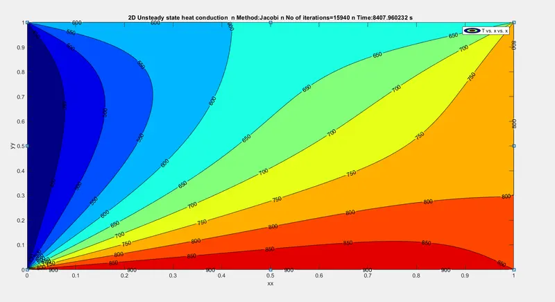
1. Jacobi method
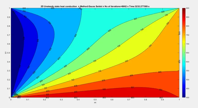
2.Gauss Seidel method
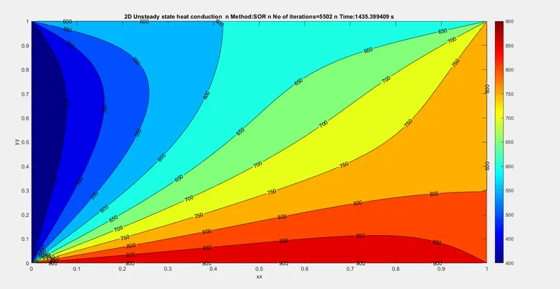
3.SOR method
transient state
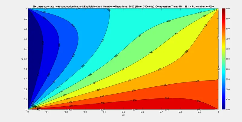
- explicit technique
2.Implicit technique
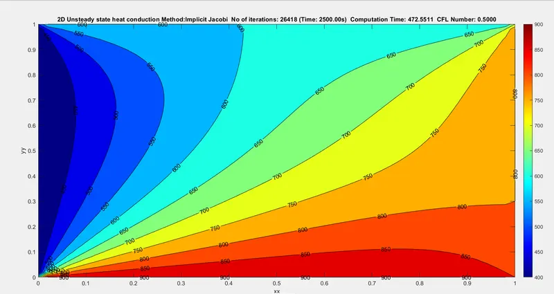
- jacobi method
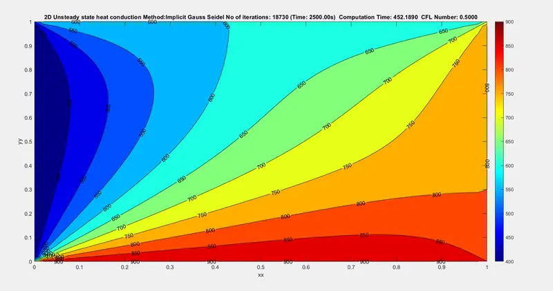
- Gauss Seidel method
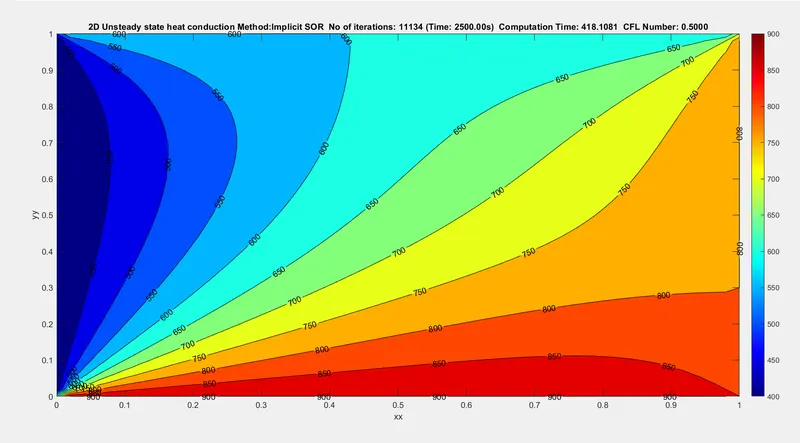
- SOR method
CONCLUSION
steady state
- as we can see from the above plots that all these methods give rise to same solutions but the number of iterations required to reach the convergence value is different in each case and time is for simulation is also different
- number of iterations: Jacobi > Gauss Seidel > SOR
- time required for simulation :Jacobi > Gauss Seidel > SOR
- Using different iterative solvers won't give us different results as the equation on which the methods are used remains the same
transient state
- as we can see from the above plots that all these methods give rise to same solutions but the number of iterations requiredto reach the convergence value is different in each case
- number of iterations: Explicit > Jacobi > Gauss Seidel > SOR