Challenge

Week 3.5 - Deriving 4th order approximation of a 2nd order derivative using Taylor Table method

KKhatu Isha Sudhir8 Jul 2022

OBJECTIVE

To derive the following 4th order approximations of the second-order derivative.

1. Central difference

2. Skewed right-sided difference

3. Skewed left-sided difference

to prove that skewed schemes used are fourth-order accurate

REPORT

1. 4th order approximations of the second-order derivative using Central difference

Number of nodes in central difference(CD) = p-q+1

where,

p-order of derivative i.e p= 2

q-order of approximation i.e q=4

`therefore`Number of nodes in CD = 2+4-1=5 ,(i.e.`(i-2),(i-1),(i),(i+1),(i+2)`)

hypothetical equation: `(del^2u)/(delx^2) =af(i-2)+bf(i-1)+cf(i)+df(i+1)+ef(i+2)` ...........................(1)

expanding each term using taylor's series-

1.`af(i-2)=a*f(i)-a*(2Deltax)(f'(i))/(1!)+a*(2Deltax)^2(f''(i))/2!-a(2Delta)^3(f''(x))/3!+a(2Deltax)^4(f^(iv)(i))/(4!)-a(2Deltax)^5(f^(v)(x))/(5!)+a(2Deltax)^6(f^(vi)(i))/(6!)`

2.`b*f(i-1)=b*f(i)-b(Deltax)(f'(i))/(1!)+b*(Deltax)^2(f''(i))/2!-b(Deltax)^3(f''(x))/3!+b(Deltax)^4(f^(iv)(i))/(4!)-b(Deltax)^5(f^(v)(x))/(5!)+b(Deltax)^6(f^(vi)(i))/(6!)`

3. `d*f(i+1)=d*f(i)+d(Deltax)(f'(i))/(1!)+d*(Deltax)^2(f''(i))/2!+d(Deltax)^3(f''(x))/3!+d(Deltax)^4(f^(iv)(i))/(4!)+d(Deltax)^5(f^(v)(x))/(5!)+d(Deltax)^6(f^(vi)(i))/(6!)`

4.`ef(i+2)=e*f(i)+e*(2Deltax)(f'(i))/(1!)+e*(2Deltax)^2(f''(i))/2!+e(2Delta)^3(f''(x))/3!+e(2Deltax)^4(f^(iv)(i))/(4!)+e(2Deltax)^5(f^(v)(x))/(5!)+e(2Deltax)^6(f^(vi)(i))/(6!)`

`ef(i+2)=ef(i)+2e(Deltax)f'(i)+4*(e/2)f''(i)(Deltax)^2+8(e/6)f'''(i)(Deltax)^3+2(e/3)f^(iv)(i)(Deltax)^4+4(e/15)f^(v)(i)(Deltax)^5+4(e/45)f^(vi)(Delatx)^6+...........................`

all the above equations are represented in taylor's table

	`f(i)`	`f'(i)(Delatx)`	`f''(i)(Deltax)^2`	`f'''(i)(Deltax)^3`	`f''''(i)(Deltax)^4`	`f'''''(Deltax)^5`	`f''''''(Deltax)^6`
af(i-2)	a	-2a	4a/2	-8a/6	2a/3	-4a/15	4a/45
bf(i-1)	b	-b	b/2	-b/6	b/24	-b/120	b/720
cf(i)	c	0	0	0	0	0	0
df(i+1)	d	d	d/2	d/6	d/24	d/120	d/720
ef(i+2)	e	2e	4e/2	8e/6	2e/3	4e/15	4e/45
`(delta^2f)/(deltax^2) =`Sum of all above terms	0	0	1	0	0	ignored	ignored

only the second derivative of function is to be soved ,sum of coefficients of `f''(i)(Deltax)^2`is only equal to 1 and rest all are equal to zero.since we require only 5 equations to find the 5 coefficients , last two columns are not taken into consideration and are ignored

therefore , we get

a+b+c+d+e=0

-2ab+d+2e=0

4a/2+b/2+d/2+4e/2=1

-8a/6-b/6+d/6+8e/6=0

2a/3+b/24+d/24+2e/3=0

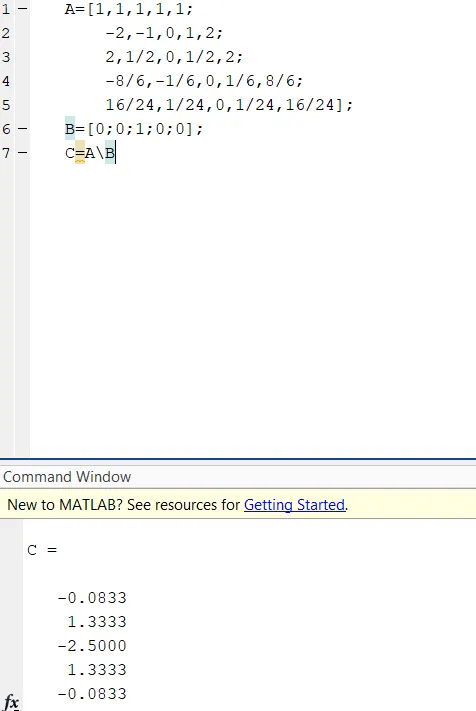
converting these equations into AX=B matrix form

`[[1,1,1,1,1],[-2,-1,0,1,2],[4/2,1/2,0,1/2,4/2],[-8/6,-1/6,0,1/6,8/6],[2/3,1/24,0,1/24,2/3]]*[[a],[b],[c],[d],[e]]=[[0],[0],[1],[0],[0]]`

solving the matrix

a=-1/12

b=4/3

c=-5/2

d=4/3

e=-1/12

hence

a=e

and

b=d

2. Skewed right side difference

Number of nodes in right side skewed = p+q

where,

p-order of derivative i.e p= 2

q-order of approximation i.e q=4

`therefore`Number of nodes in CD = 2+4 =5 ,(i.e.`(i),(i+1),(i+2),(i+3),(i+4),(i+5)``

`hypothetical equation: `(del^2u)/(delx^2) =af(i)+bf(i+1)+cf(i+2)+df(i+3)+ef(i+4)+gf(i+5)` ...........................(1`

expanding each term using taylor's series-

1.`.`af(i)=a*f(i)`

`2`.`b*f(i+1)=b*f(i)+b(Deltax)(f'(i))/(1!)+b*(Deltax)^2(f''(i))/2!+b(Deltax)^3(f''(x))/3!+b(Deltax)^4(f^(iv)(i))/(4!)+b(Deltax)^5(f^(v)(x))/(5!)+b(Deltax)^6(f^(vi)(i))/(6!)`

3.`c*f(i+2)=c*f(i)+c*(2*Deltax)(f'(i))/(1!)+c*(2*Deltax)^2(f''(i))/2!+c*(2*Deltax)^3(f''(x))/3!+c*(2*Deltax)^4(f^(iv)(i))/(4!)+c*(2*Deltax)^5(f^(v)(x))/(5!)+c*(2*Deltax)^6(f^(vi)(i))/(6!)`

4.`d*f(i+3)=d*f(i)+d*(3*Deltax)(f'(i))/(1!)+d*(3*Deltax)^2(f''(i))/2!+d*(3*Deltax)^3(f''(x))/3!+d*(3*Deltax)^4(f^(iv)(i))/(4!)+d*(3*Deltax)^5(f^(v)(x))/(5!)+d*(3*Deltax)^6(f^(vi)(i))/(6!)`

5.`e*f(i+4)=e*f(i)+e*(4*Deltax)(f'(i))/(1!)+e*(4*Deltax)^2(f''(i))/2!+e*(4*Deltax)^3(f''(x))/3!+e*(4*Deltax)^4(f^(iv)(i))/(4!)+e*(4*Deltax)^5(f^(v)(x))/(5!)+e*(4*Deltax)^6(f^(vi)(i))/(6!)`

6.`g*f(i+5)=g*f(i)+g*(5*Deltax)(f'(i))/(1!)+g*(5*Deltax)^2(f''(i))/2!+g*(5*Deltax)^3(f''(x))/3!+g*(5*Deltax)^4(f^(iv)(i))/(4!)+g*(5*Deltax)^5(f^(v)(x))/(5!)+g*(5*Deltax)^6(f^(vi)(i))/(6!)`

all the above equations are represented in taylor's table

	`f(i)`	`f'(i)(Delatx)`	`f''(i)(Deltax)^2`	`f'''(i)(Deltax)^3`	`f''''(i)(Deltax)^4`	`f'''''(Deltax)^5`	`f''''''(Deltax)^6`
af(i)	a	0	0	0	0	0	0
bf(i+1)	b	b	b/2	b/6	b/24	b/120	b/720
cf(i+2)	c	2c	4c/2	8c/6	16c/24	32c/120	64c/720
df(i+3)	d	3d	9d/2	27d/6	81d/24	243d/120	729d/720
ef(i+4)	e	4e	16e/2	64e/6	256e/24	1024e/120	4096e/720
gf(i+5)	g	5g	25g/2	125g/6	625g/24	3125g/120	15625g/720
`(delta^2f)/(deltax^2) =`Sum of all above terms	0	0	1	0	0	0	ignored

therefore , we get

`a+b+c+d+e+g=0`

`b+2c+3d+4e+5g=0`

`b/2+4*c/2+9*d/2+16*e/2+25*g/2=1`

`b/6+8*c/6+27*d/6+64*e/6+125*g/6=0`

`b/24+16*c/24+81*d/24+256*e/24+625*g/24=0`

`b/120+32*c/120+243*d/120+1024*e/120+3125*g/120=0`

`b/720+64*c/720+729*d/720+4096*e/720+15625*g/720=0`

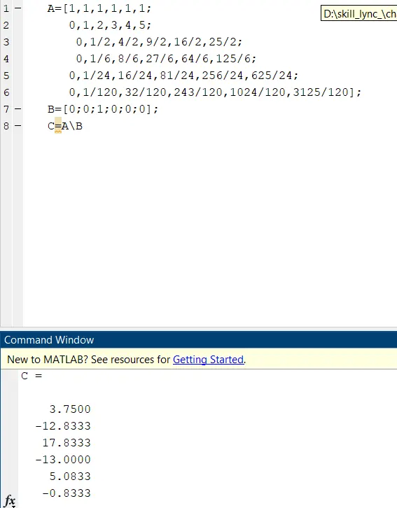
converting these equations into AX=B matrix form

`[[1,1,1,1,1,1],[0,1,2,3,4,5],[0,1/2,4/2,9/2,16/2,25/2],[0,1/6,8/6,27/6,64/6,125/6],[0,1/24,16/24,81/24,256/24,625/24],[0,1/120,32/120,243/120,1024/120,3125/120],[0,1/720,64/720,729/720,4096/720,15625/720]]*[[a],[b],[c],[d],[e],[g]]=[[0],[0],[1],[0],[0],[0]]`

solving the matrix

a=15/4

b=-77/6

c=107/6

d=-13

e=61/12

g=-5/6

hence

a=e

and

b=d

3. Skewed left side difference

Number of nodes in right side skewed = p+q

where,

p-order of derivative i.e p= 2

q-order of approximation i.e q=4

`therefore`Number of nodes in CD = 2+4 =5 ,(i.e.`(i),(i-1),(i-2),(i-3),(i-4),(i-5)`

`hypothetical equation: `(del^2u)/(delx^2) =af(i)+bf(i-1)+cf(i-2)+df(i-3)+ef(i-4)+gf(i-5)` ...........................(1)`

expanding each term using taylor's series-

1.`.`af(i)=a*f(i)`

2.`b*f(i-1)=b*f(i)-b*(Deltax)(f'(i))/(1!)+b*(Deltax)^2(f''(i))/2!-b*(Deltax)^3(f''(x))/3!+b*(Deltax)^4(f^(iv)(i))/(4!)-b*(Deltax)^5(f^(v)(x))/(5!)+b*(Deltax)^6(f^(vi)(i))/(6!)`

3.`c*f(i-2)=c*f(i)-c*(2*Deltax)(f'(i))/(1!)+c*(2*Deltax)^2(f''(i))/2!-c*(2*Deltax)^3(f''(x))/3!+c*(2*Deltax)^4(f^(iv)(i))/(4!)-c*(2*Deltax)^5(f^(v)(x))/(5!)+c*(2*Deltax)^6(f^(vi)(i))/(6!)`

4.`d*f(i-3)=d*f(i)-d*(3*Deltax)(f'(i))/(1!)+d*(3*Deltax)^2(f''(i))/2!-d*(3*Deltax)^3(f''(x))/3!+d*(3*Deltax)^4(f^(iv)(i))/(4!)-d*(3*Deltax)^5(f^(v)(x))/(5!)+d*(3*Deltax)^6(f^(vi)(i))/(6!)`

5.`e*f(i-4)=e*f(i)-e*(4*Deltax)(f'(i))/(1!)+e*(4*Deltax)^2(f''(i))/2!-e*(4*Deltax)^3(f''(x))/3!+e*(4*Deltax)^4(f^(iv)(i))/(4!)-e*(4*Deltax)^5(f^(v)(x))/(5!)+e*(4*Deltax)^6(f^(vi)(i))/(6!)`

6.`g*f(i-5)=g*f(i)-g*(5*Deltax)(f'(i))/(1!)+g*(5*Deltax)^2(f''(i))/2!-g*(5*Deltax)^3(f''(x))/3!+g*(5*Deltax)^4(f^(iv)(i))/(4!)-g*(5*Deltax)^5(f^(v)(x))/(5!)+g*(5*Deltax)^6(f^(vi)(i))/(6!)`

all the above equations are represented in taylor's table

	`f(i)`	`f'(i)(Delatx)`	`f''(i)(Deltax)^2`	`f'''(i)(Deltax)^3`	`f''''(i)(Deltax)^4`	`f'''''(Deltax)^5`	`f''''''(Deltax)^6`
af(i)	a	0	0	0	0	0	0
bf(i-1)	b	-b	b/2	-b/6	b/24	-b/120	b/720
cf(i-2)	c	-2c	4c/2	-8c/6	16c/24	-32c/120	64c/720
df(i-3)	d	-3d	9d/2	-27d/6	81d/24	-243d/120	729d/720
ef(i-4)	e	-4e	16e/2	-64e/6	256e/24	-1024e/120	4096e/720
gf(i-5)	g	-5g	25g/2	-125g/6	625g/24	-3125g/120	15625g/720
`(delta^2f)/(deltax^2) =`Sum of all above terms	0	0	1	0	0	0	ignored

therefore , we get

`a+b+c+d+e+g=`

`-b-2c-3d-4e-5g=1`

`b/2+4*c/2+9*d/2+16*e/2+25*g/2=0`

`-b/6-8*c/6-27*d/6-64*e/6-125*g/6=0`

`b/24+16*c/24+81*d/24+256*e/24+625*g/24=0`

`-b/120-32*c/120-243*d/120-1024*e/120-3125*g/120=0`

`b/720+64*c/720+729*d/720+4096*e/720+15625*g/720=0`

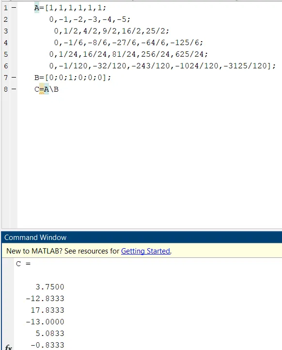
converting these equations into AX=B matrix form

`[[1,1,1,1,1,1],[0,-1,-2,-3,-4,-5],[0,1/2,4/2,9/2,16/2,25/2],[0,-1/6,-8/6,-27/6,-64/6,-125/6],[0,1/24,16/24,81/24,256/24,625/24],[0,-1/120,-32/120,-243/120,-1024/120,-3125/120],[0,1/720,64/720,729/720,4096/720,15625/720]]*[[a],[b],[c],[d],[e],[g]]=[[0],[0],[1],[0],[0],[0]]`

solving the matrix

a=15/4

b=-77/6

c=107/6

d=-13

e=61/12

g=-5/6

hence

a=e

and

b=d

CODE

main code

close all 
clear all
clc

%analytical_function=f(x)=exp(x)*cos(x)
%analytical_derivative=f''(x)=-2*exp(x)*sin(x)

x=pi/3;
dx = linspace(pi/400,pi/4,50);

for i=1:length(dx)
    central_differencing_scheme_error(i) = central_difference(x,dx(i));
    right_skewed_scheme_error(i) = right_skewed_difference(x,dx(i));
    left_skewed_scheme_error(i) = left_skewed_difference(x,dx(i)); 
end


%plotting the error graphs
figure(1)
loglog(dx,central_differencing_scheme_error,'color','b','marker','diamond');
hold on
loglog(dx,right_skewed_scheme_error,'color','g','marker','*');
hold on
loglog(dx,left_skewed_scheme_error,'color','r','marker','.');
xlabel('grid size')
ylabel('absolute error')
legend('Central difference of 4th order','Skewed right sided difference of 4th order','Skewed left sided difference of 4th order')
title('COnsistency of different scheme')

function code for central difference

function central_error=central_difference(x,dx)
%analytical_derivative
analytical_derivative=-2*exp(x)*sin(x);
a=(-1/12);
b=(4/3);
c=(-5/2);
d=(4/3);
e=(-1/12);
central_difference=(a*exp(x-2*dx)*cos(x-2*dx)+b*exp(x-dx)*cos(x-dx)+c*exp(x)*cos(x)+d*exp(x+dx)*cos(x+dx)+e*exp(x+2*dx)*cos(x+2*dx))/(dx^2);
central_error=abs(central_difference-analytical_derivative);
end

function code for left skewed difference

function left_error=left_skewed_difference(x,dx)
%analytical_derivative
analytical_derivative=-2*exp(x)*sin(x);
a=(15/4);
b=(-77/6);
c=(107/6);
d=(-13);
e=(61/12);
g=(-5/6);
left_scheme=(a*exp(x)*cos(x)+b*exp(x-dx)*cos(x-dx)+c*exp(x-2*dx)*cos(x-2*dx)+d*exp(x-3*dx)*cos(x-3*dx)+e*exp(x-4*dx)*cos(x-4*dx)+g*exp(x-5*dx)*cos(x-5*dx))/(dx^2);
left_error=abs(left_scheme-analytical_derivative);
end

function code for right skewed difference

function right_error=right_skewed_difference(x,dx)
%analytical_derivative
analytical_derivative=-2*exp(x)*sin(x);
a=(15/4);
b=(-77/6);
c=(107/6);
d=(-13);
e=(61/12);
g=(-5/6);
right_scheme=(a*exp(x)*cos(x)+b*exp(x+dx)*cos(x+dx)+c*exp(x+2*dx)*cos(x+2*dx)+d*exp(x+3*dx)*cos(x+3*dx)+e*exp(x+4*dx)*cos(x+4*dx)+g*exp(x+5*dx)*cos(x+5*dx))/(dx^2);
right_error=abs(right_scheme-analytical_derivative);
end

CODE EXPLANATION

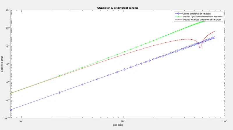
The aim is to compare three scheme by plotting it on a graph

function code is used for each scheme.this function can be called again and again in the main code .analytical derivative of `e^x.cosx`is calculated. since the question is about second order derivative,analytical derivative to be calculated is of second order.
co efficient of different scheme are calculated by converting the linear equations into matrix form AX=B and solving it by using inversion method
error calculated here is absolute error,by using the command abs and subtracting the three different schemes with analytical derivative
main code consists of three parts
1st is assigning the value of x
assigning the range for dx by using linspace command to create an array
dx is the grid size/mesh size/distance between two nodes
2nd part is creating a for loop
idea behind creating a for loop is calculate the error for three different schemes throughout the range of dx, i is counter loop variable ,it keeps on updating the value of dx
3rd part is to create a plot buy using the loglog

OUTPUT

CONCLUSION

error is least in case of central differnce hence more accurate as compared to other schemes
as grid size increases,error also increases

order of accuracy

for central difference =No. of nodes-order of derivative+1=5-2+1=4
for skewed scheme=No. of nodes-order of derivative=6-2=4

SKEWED V/S CENTRAL DIFFERENCE

at boundary conditions, skewed scheme is required
except the boundary,at all other nodes in flluid domain central difference is used
in cfd mostly, the boundary conditions(b.c) are known.by applying skewed scheme to boundary nodes , value at other nodes can be calculated where central diference can bu used

Week 3.5 - Deriving 4th order approximation of a 2nd order derivative using Taylor Table method

Ship work like this
in your own course.

Talk to a career counsellor

Ship work like thisin your own course.

Talk to a career counsellor

Ship work like this
in your own course.