Week 11 - Simulation of Flow through a pipe in OpenFoam
AIM
To simulate an axi-symmetric flow by applying the wedge boundary condition. The flow is laminar and flows through a constant cross-section pipe at an inlet Reynold's number of 2100.To do a transient or steady state simulation and will validate the results with the Hagen- Poiseuille's equations for the fully developed flow.
OBJECTIVE
write code in Matlab to automate the generation of blockMeshDict file.
- Validate Hydro-dynamic length with the numerical result
- Validate the fully developed flow velocity profile with its analytical profile
- Validate maximum velocity and pressured drop for fully developed flow
- Post-process Shear stress and validate wall shear stress for fully developed flow
THEORY
HAGEN-POISEUILLE EQUATION
In nonideal fluid dynamics, the Hagen–Poiseuille equation, also known as the Hagen–Poiseuille law, Poiseuille law or Poiseuille equation, is a physical law that gives the pressure drop in an incompressible and Newtonian fluid in laminar flow flowing through a long cylindrical pipe of constant cross section.
ASSUMPTIONS
- Fluid is incompressible and Newtonian.
- Flow is laminar through pipe of constant circular cross section area having length more than its Diameter
- No acceleration of fluid in pipe
- For velocities and pipe diameters above a threshold, actual fluid flow is not laminar but turbulent, leading to larger pressure drops than calculated by the Hagen–Poiseuille equation.
Poiseuille's equation describes the pressure drop due to the viscosity of the fluid; Other types of pressure drops may still occur in a fluid (see a demonstration here). For example, the pressure needed to drive a viscous fluid up against gravity would contain both that as needed in Poiseuille's law plus that as needed in Bernoulli's equation, such that any point in the flow would have a pressure greater than zero (otherwise no flow would happen).
In standard fluid-kinetics notation:
PRESSURE DIFFERENCE
- `Deltap=(8muLQ)/(piR^4)=(8muLpiQ)/(A^2)=(32muLQ)/(piD^4)`
HYDRODYNAMIC ENTRY LENGTH
-
LE`=0.06*D*Re
SHEAR STRESS(NEWTON'S LAW OF VISCOSITY)
`tau=mu*(delu)/(dely)`
VELOCITY PROFILE

from the above equation, velocity of flow increases parabolically from wall to center of pipe
where:
- Δp is the pressure difference between the two ends,
- L is the length of pipe,
- μ is the dynamic viscosity,
- Q is the volumetric flow rate,
- R is the pipe radius,
- A is the cross section of pipe.
The equation does not hold close to the pipe entrance.
The ratio of length to radius of a pipe should be greater than one forty-eighth of the Reynolds number for the Hagen–Poiseuille law to be valid.
The Hagen–Poiseuille equation can be derived from the Navier–Stokes equations. The laminar flow through a pipe of uniform (circular) cross-section is known as Hagen–Poiseuille flow. The equations governing the Hagen–Poiseuille flow can be derived directly from the Navier–Stokes momentum equations in 3D cylindrical coordinates (r,θ,x) by making the following set of assumptions:
- The flow is steady ( ∂(...)/∂t=0 ).
- The radial and azimuthal components of the fluid velocity are zero ( ur=uθ=0 ).
- The flow is axisymmetric ( ∂(...)/∂θ=0 ).
- The flow is fully developed (∂ux/∂x=0 ). Here However, this can be proved via mass conservation, and the above assumptions.
CONSIDERATIONS
Working temperature of water=25 degree C
`therefore density(rho)=997(kg)/m^3`density
dynamic viscosity`(mu)=8.90 xx10^-4 Pa.s`
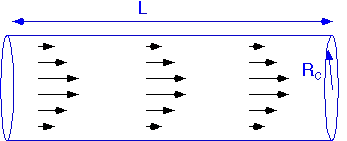
Diameter (D)=0.02m
Length of the pipe(L)=2.5m
PARAMETERS
Re=2100 ......................(given in the problem statement)
MATLAB CODE
- As the value of vertices can be calculated by resolving the components of radius.
- For this we can use file parsing method to write the blockMeshDict file in OpenFoam by writing a code in matlab,'fprintf' command is used to print as parameters like vertices,blocks,boundary(inlet,outlet,front,back,pipewall,axis)
Main code
- Input variables are assigned like
>reynolds number(given in the problem statement)
>Apex angle of wedge
>Diameter of the pipe
>Radius of the pipe
>density of fluid
>dynamic viscosity
>Total length of the pipe
>entrance length of the pipe
- Function code'blockMesh' is being called out
- After running the simulation on OpenFoam and getting its result from paraView .Now we have to compare the analytical and numerical values and compare its result in plot
- for this the analytical values are being calculated
- average velocity of pipe is calculated
- velocity at different points from centre of pipe is calculated
- pressure drop across length of pipe is calculated
- Wall shear stress is calculated
- now the values obtained in paraView is being imported to matlab by opening the csv file in the current folder
- And 'fopen' command is used in the code to open the csv file
- the data is for 1000 points in the csv file, so a for loop is created from 1 to 1000 to get the thousand valus of velocity
- B variable is used to command 'fgetl' that Read line(s) from file, discard newline character
- C variable is used to spilt B into rows having ','between two value
- U_mag is in the 13th column ,v_n(numerical value) is assigned the 13th column of C for every change in value of i
- now vn variable is updated by using the command 'str2double(vn)' converts an array of character vectors into a numeric array
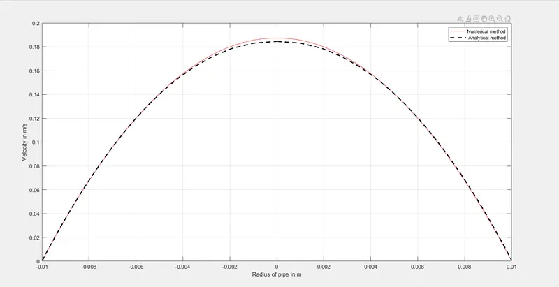
- now to compare the results vr ,vn is plotted on Y-axis and radius on X-axis
clear all
close all
clc

%%Variables
R=2100;               %Reynold's number
theta=input('Enter the wedge angle = ');       %wedge angle(in degrees)
D=0.02;            %Diameter of the pipe (m)
r=D/2;             %Radius of the pipe(m)
rho=997;           %Density(kg/m^3)
mu = 8.90e-4;       %Dynamic Viscosity
L=2.5;                %Total length of the pipe(m)
Le=0.058*R*D;      %Entrance length

nx = 20;               %cells along x
ny = 1;                %cells along y
nz = 500;              %cells along z

%%BlockMeshDict
[f1]=blockMesh(r,theta,L,nx,ny,nz);

%%analytical values
v_avg=(R*mu)/(rho*D);          %average velocity


x=linspace(-r,r,1000);     %distance from center of pipe to the circumference


%velocity at different radius in fully developed region
vr=2*v_avg*(1-(x.^2/r^2));


v_max=2*v_avg;             %velocity at center of pipe

L_p=linspace(0,L,1000);          %length of pipe

%pressure drop across the length of pipe
P_d=(32*mu.*L_p*v_avg)/D^2;
P_d=fliplr(P_d);

f=64/R;%darcy friction factor
tau_a=(f/4)*((rho*v_avg^2)/2);%%Wall Shear Stress

%Reading and Extracting Velocity Data From ParaView
f2=fopen('vel_ss.csv','r');
A=fgetl(f2);
for i=1:1000
    B=fgetl(f2);
    C=strsplit(B,',');
    v_n(i)=C(13);

end
v_n=str2double(v_n);


%%[1]-Plotting - Velocity comparison from analytical method and numerical method
figure(1)
plot(x,vr,'r')
hold on
plot(x,v_n,'--','color','k','linewidth',2)
xlabel('Radius of pipe in m')
ylabel('Velocity in m/s')
legend('Numerical method',' Analytical method')
grid on


%Error
E_max=max(max(abs(vr-v_n)));
function code for blockMeshDict file
- Since the pipe is a axi-symmetric,there is no need to simulate the entire pipe.wedge having apex angle less than 5 degrees can be used making no changes in the final result.
- the below figure is the schematic representation of the wedge
- X-axis is bisecting the apex angle of the wedge
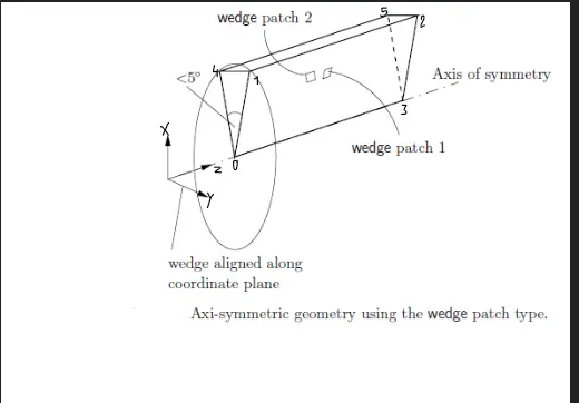
- vertice 0 is taken as the origin of the entire system v0=(0,0,0)
- vertice 1`=(rcos(theta/2),rsin(theta/2),0)`
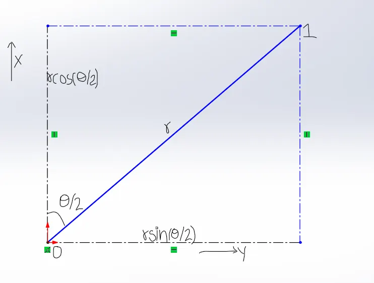
- vertice 2=`(rcos(theta/2),rsin(theta/2),L)`
- vertice 3=`(0,0,L)`
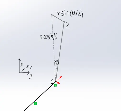
- vertice 4=(`rcos(theta/2),-rsin(theta/2),0`)
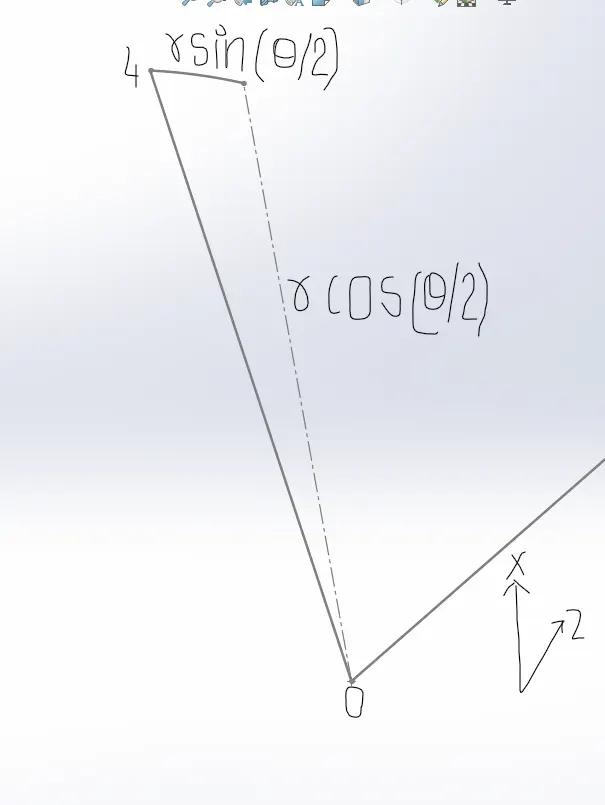
- vertice 5=`(rcos(theta/2),-rsin(theta/2),L)`
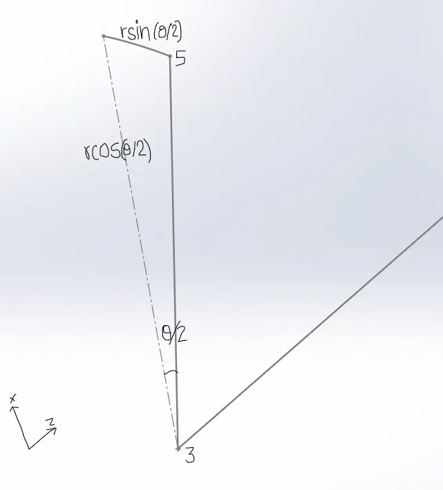
- function code is used for generation of blockMeshDict file
- It starts by writing 'fopen' command
- before define any vertices,boundary .,header information as comment is printed which is not executable in OpenFoam
- to have uniformity in dimensions , all type of length is converted to meters
- Vertices are defined as stated above in the figures
- Mesh of pipe includes a new feature called as the wedge(block having less than 8 vertices)
- hexahedral meshing is generated
- vertices are numbered according to right hand thumb rule
- vertice 4-1 and vertice 5-2 are curved so it it defined in edges by arc
- since there is no physical wall in (0-1-2-3) and(0-4-5-3),and there exists a patch wedge in the two faces thta indicates the presence of axi-symmetry
function[f1]=blockMesh(r,theta,L,nx,ny,nz)
%%File writing
line1 = '/*--------------------------------*- C++ -*----------------------------------*\';
line2 = '| =========                 |                                                 |';
line3 = '| \\      /  F ield         | OpenFOAM: The Open Source CFD Toolbox           |';
line4 = '|  \\    /   O peration     | Version:  v2012                                 |';
line5 = '|   \\  /    A nd           | Website:  www.openfoam.com                      |';
line6 = '|    \\/     M anipulation  |                                                 |';
line7 = '\*---------------------------------------------------------------------------*/';

%file open
f1 = fopen('blockMeshDict','w');

%To write header
fprintf(f1,'%s\n',line1);
fprintf(f1,'%s\n',line2);
fprintf(f1,'%s\n',line3);

fprintf(f1,'%s\n',line4);
fprintf(f1,'%s\n',line5);
fprintf(f1,'%s\n',line6);
fprintf(f1,'%s\n',line7);

%To write the dictionary
fprintf(f1,'FoamFile \n');
fprintf(f1,'{ \n');
fprintf(f1,'    version      2.0;\n');
fprintf(f1,'    format       ascii;\n');
fprintf(f1,'    class        dictionary;\n');
fprintf(f1,'    object       blockMeshDict;\n');
fprintf(f1,'}');
fprintf(f1,'// * * * * * * * * * * * * * * * * * * * * * * * * * * * * * * * * * * * * * //');
fprintf(f1,'\n');

% Note: As all the calculated variables are in meter(m), keeping scale to
% be as one (1).

fprintf(f1,'convertToMeters 1;\n\n');

%Vertices
fprintf(f1,'vertices\n');
fprintf(f1,'(\n');

fprintf(f1,'\t (0 0 0)\n');
fprintf(f1,('\t (%f %f 0)\n'),r*cosd(theta/2),r*sind(theta/2));
fprintf(f1,('\t (%f %f %f)\n'),r*cosd(theta/2),r*sind(theta/2),L);
fprintf(f1,('\t (0 0 %f)\n'),L);
fprintf(f1,('\t (%f %f 0)\n'),r*cosd(theta/2),-r*sind(theta/2));
fprintf(f1,('\t (%f %f %f)\n);\n\n'),r*cosd(theta/2),-r*sind(theta/2),L);

%Write block
fprintf(f1,'blocks\n(\n');
fprintf(f1,('hex (0 4 1 0 3 5 2 3) (%d %d %d) simpleGrading (0.2 1 1)\n);\n\n'),nx,ny,nz);

%Edges
fprintf(f1,'edges\n(\n');
fprintf(f1,'\t arc 4 1 (0 %f 0)\n',r);
fprintf(f1,'\t arc 5 2 (%f %f 0)\n);\n\n',L,r);

%Boundary
fprintf(f1,'boundary\n(\n');
%Inlet

fprintf(f1,'     inlet\n');
fprintf(f1,'     {\n');
fprintf(f1,'           type patch;\n');
fprintf(f1,'           faces\n');
fprintf(f1,'           (\n');
fprintf(f1,'               (0 4 1 0)\n');
fprintf(f1,'           );\n');
fprintf(f1,'     }\n');
%outlet
fprintf(f1,'     outlet\n');
fprintf(f1,'     {\n');
fprintf(f1,'           type patch;\n');
fprintf(f1,'           faces\n');
fprintf(f1,'           (\n');
fprintf(f1,'               (3 5 2 3)\n');
fprintf(f1,'           );\n');
fprintf(f1,'      }\n');
%Front wedge
fprintf(f1,'      front\n');
fprintf(f1,'      {\n');
fprintf(f1,'            type wedge;\n');
fprintf(f1,'            faces\n');
fprintf(f1,'            (\n');
fprintf(f1,'                (0 1 2 3)\n');
fprintf(f1,'            );\n');
fprintf(f1,'      }\n');
%Back wedge
fprintf(f1,'      back\n');
fprintf(f1,'      {\n');
fprintf(f1,'            type wedge;\n');
fprintf(f1,'            faces  \n');
fprintf(f1,'            (\n');
fprintf(f1,'                (0 3 5 4)\n');
fprintf(f1,'            );\n');
fprintf(f1,'      }\n');
%Top wall
fprintf(f1,'      pipewall\n');
fprintf(f1,'      {\n');
fprintf(f1,'            type wall;\n');
fprintf(f1,'            faces\n');
fprintf(f1,'            (\n');
fprintf(f1,'                (1 4 5 2)\n');
fprintf(f1,'            );\n');
fprintf(f1,'     }\n');
%Bottom wall
fprintf(f1,'     axis\n');
fprintf(f1,'     {\n');
fprintf(f1','          type empty;\n');
fprintf(f1,'           faces\n');
fprintf(f1,'           (\n');
fprintf(f1,'               (0 3 3 0)\n');
fprintf(f1,'           );\n');
fprintf(f1,'     }\n');

fprintf(f1,');\n\n');
fprintf(f1,'margePatchPairs\n');
fprintf(f1,'(\n');
fprintf(f1,');\n\n');
fprintf(f1,'// * * * * * * * * * * * * * * * * * * * * * * * * * * * * * * * * * * * * * //');
fclose(f1);
end
OpenFoam
blockMeshDict
/*--------------------------------*- C++ -*----------------------------------*\
| =========                 |                                                 |
| \\      /  F ield         | OpenFOAM: The Open Source CFD Toolbox           |
|  \\    /   O peration     | Version:  v2012                                 |
|   \\  /    A nd           | Website:  www.openfoam.com                      |
|    \\/     M anipulation  |                                                 |
\*---------------------------------------------------------------------------*/
FoamFile
{
    version      2.0;
    format       ascii;
    class        dictionary;
    object       blockMeshDict;
}// * * * * * * * * * * * * * * * * * * * * * * * * * * * * * * * * * * * * * //
convertToMeters 1;

vertices
(
	 (0 0 0)
	 (0.009997 0.000262 0)
	 (0.009997 0.000262 2.500000)
	 (0 0 2.500000)
	 (0.009997 -0.000262 0)
	 (0.009997 -0.000262 2.500000)
);

blocks
(
hex (0 4 1 0 3 5 2 3) (20 1 500) simpleGrading (0.2 1 1)
);

edges
(
	 arc 4 1 (0 0.010000 0)
	 arc 5 2 (2.500000 0.010000 0)
);

boundary
(
     inlet
     {
           type patch;
           faces
           (
               (0 4 1 0)
           );
     }
     outlet
     {
           type patch;
           faces
           (
               (3 5 2 3)
           );
      }
      front
      {
            type wedge;
            faces
            (
                (0 1 2 3)
            );
      }
      back
      {
            type wedge;
            faces
            (
                (0 3 5 4)
            );
      }
      pipewall
      {
            type wall;
            faces
            (
                (1 4 5 2)
            );
     }
     axis
     {
          type empty;
           faces
           (
               (0 3 3 0)
           );
     }
);

margePatchPairs
(
);

// * * * * * * * * * * * * * * * * * * * * * * * * * * * * * * * * * * * * * //
controlDict
/*--------------------------------*- C++ -*----------------------------------*\
| =========                 |                                                 |
| \\      /  F ield         | OpenFOAM: The Open Source CFD Toolbox           |
|  \\    /   O peration     | Version:  v2012                                 |
|   \\  /    A nd           | Website:  www.openfoam.com                      |
|    \\/     M anipulation  |                                                 |
\*---------------------------------------------------------------------------*/
FoamFile
{
    version     2.0;
    format      ascii;
    class       dictionary;
    location    "system";
    object      controlDict;
}
// * * * * * * * * * * * * * * * * * * * * * * * * * * * * * * * * * * * * * //

application     icoFoam;

startFrom       latestTime;			// startTime, or to resume, latestTime

startTime       0;

stopAt          endTime;

endTime         30;

deltaT          0.02;

writeControl    runTime;			// or timeStep

writeInterval   0.5;				// while using timeStep, writing an oputput folder every writeInterval*deltaT or else the value specified

purgeWrite      0;				// retain the last specified number of files...to retain all 0

writeFormat     ascii;

writePrecision  6;

writeCompression off;

timeFormat      general;

timePrecision   6;

runTimeModifiable true;


// ************************************************************************* //
Initial Conditions
velocity
At the inlet of the pipe ,initial velocity in the Z directions is given.This velocity is the average velocity of the pipe that is calculated in the main code.


/*--------------------------------*- C++ -*----------------------------------*\
| =========                 |                                                 |
| \\      /  F ield         | OpenFOAM: The Open Source CFD Toolbox           |
|  \\    /   O peration     | Version:  v2012                                 |
|   \\  /    A nd           | Website:  www.openfoam.com                      |
|    \\/     M anipulation  |                                                 |
\*---------------------------------------------------------------------------*/
FoamFile
{
    version     2.0;
    format      ascii;
    class       volVectorField;
    object      U;
}
// * * * * * * * * * * * * * * * * * * * * * * * * * * * * * * * * * * * * * //

dimensions      [0 1 -1 0 0 0 0];

internalField   uniform (0 0 0);

boundaryField
{
    inlet
    {
        type            fixedValue;
        value           uniform (0 0 0.0937);
    }

    outlet
    {
        type            zeroGradient;
    }

    front
    {
        type            wedge;
    }
    back
    {
        type            wedge;
    }

    axis
    {
        type            empty;
    }

    pipewall
    {
        type            noSlip;
    }

}

// ************************************************************************* //
pressure
/*--------------------------------*- C++ -*----------------------------------*\
| =========                 |                                                 |
| \\      /  F ield         | OpenFOAM: The Open Source CFD Toolbox           |
|  \\    /   O peration     | Version:  v2012                                 |
|   \\  /    A nd           | Website:  www.openfoam.com                      |
|    \\/     M anipulation  |                                                 |
\*---------------------------------------------------------------------------*/
FoamFile
{
    version     2.0;
    format      ascii;
    class       volScalarField;
    object      p;
}
// * * * * * * * * * * * * * * * * * * * * * * * * * * * * * * * * * * * * * //

dimensions      [0 2 -2 0 0 0 0];

internalField   uniform 0;

boundaryField
{
    inlet
    {
        type            zeroGradient;
    }

    outlet
    {
        type            fixedValue;
        value           uniform 0;
    }

    front
    {
        type            wedge;
    }

    back
    {
        type           wedge;
    }

    axis
    {
        type           empty;
    }

    pipewall
    {
        type           zeroGradient;
    }

}

// ************************************************************************* //
transportProperties
In openFoam,every tutorial has three files namely 0,constant and system.The 'constant' file stores transport properties file in notepad. this has value `nu`i.e,kinetic viscosity.we to convert the dynamic viscosity that we have considered for this problem statement into kinetic viscosity by using the below formula
`nu=mu/rho`
where `nu`-kinetic viscosity
`mu`-dynamic viscosity=8.90e-4
`rho`-density=997

/*--------------------------------*- C++ -*----------------------------------*\
| =========                 |                                                 |
| \\      /  F ield         | OpenFOAM: The Open Source CFD Toolbox           |
|  \\    /   O peration     | Version:  v2012                                 |
|   \\  /    A nd           | Website:  www.openfoam.com                      |
|    \\/     M anipulation  |                                                 |
\*---------------------------------------------------------------------------*/
FoamFile
{
    version     2.0;
    format      ascii;
    class       dictionary;
    location    "constant";
    object      transportProperties;
}
// * * * * * * * * * * * * * * * * * * * * * * * * * * * * * * * * * * * * * //

nu              [0 2 -1 0 0 0 0] 8.9268e-07;


// ************************************************************************* //
OUTPUT
Mesh of the wedge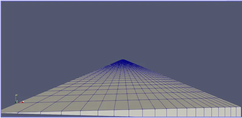
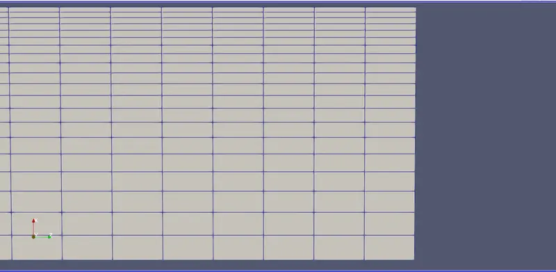
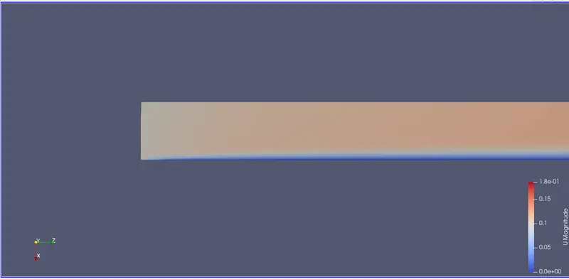
Velocity at the entrance length at a steady state
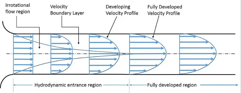
The layer in which the shearing viscous forces are significant, is called the boundary layer. This boundary layer is a hypothetical concept. It divides the flow in pipe into two regions:
- Boundary layer region: The region in which viscous effects and the velocity changes are significant.
- The irrotational (core) flow region: The region in which viscous effects and velocity changes are negligible, also known as the inviscid core.
When the fluid just enters the pipe, the thickness of the boundary layer gradually increases from zero moving in the direction of fluid flow and eventually reaches the pipe center and fills the entire pipe. This region from the entrance of the pipe to the point where the boundary layer covers the entire pipe is termed as the hydrodynamic entrance region and the length of the pipe in this region is termed as the hydrodynamic entry length. In this region, the velocity profile develops and thus the flow is called the hydrodynamically developing flow. After this region, the velocity profile is fully developed and continues unchanged. This region is called the hydrodynamically fully developed region. But this is not the fully developed fluid flow until the normalized temperature profile also becomes constant.
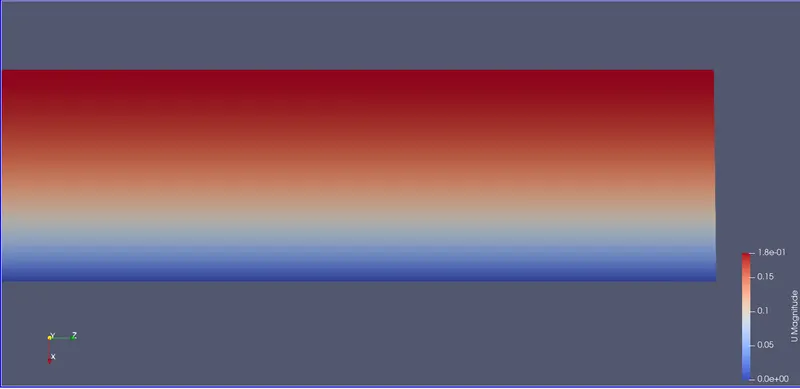
In case of laminar flow, the velocity profile in the fully developed region is parabolic but in the case of turbulent flow it gets a little flatter due to vigorous mixing in radial direction and eddy motion.
The velocity profile remains unchanged in the fully developed region.
Shear stress at entrance length at 0.1s(simulation time)
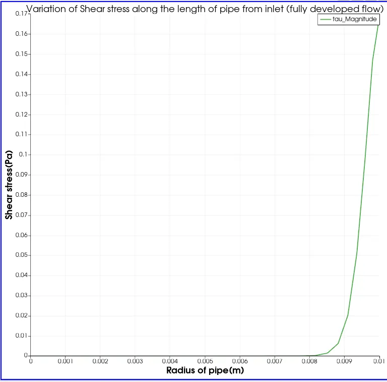
Shear stress at entrance length at 30 s(simulation time)
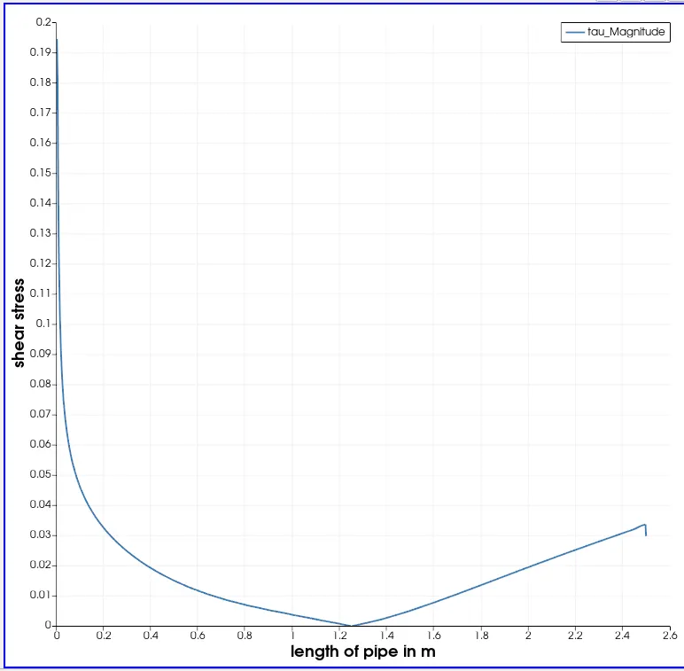
In the hydrodynamic entrance region, the wall shear stress is highest at the pipe inlet, where the boundary layer thickness is the smallest. Shear stress decreases along the flow direction. That is why the pressure drop is highest in the entrance region of a pipe, which increases the average friction factor for the whole pipe. This increase in the friction factor is negligible for long pipes.
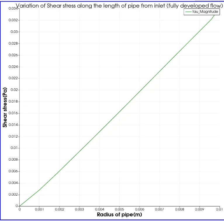
In a fully developed region, the pressure gradient and the shear stress in flow are in balance
Velocity at inlet
in the below figure , shear stress along the surface of the pipe is decreasing as the fluid moves forward
Velocity at outlet
this is a fully developed flow as velocity and shear stress remains constant
after updating the 0,system, constant files in OpenFoam,the simulation is opened in ParaView. since the simulation is on pipe we need to create a mirror of the simulation of wedge.
this is done by using 'Reflect' in the paraview .
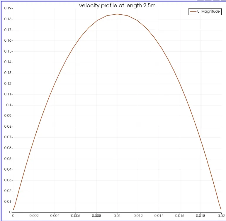
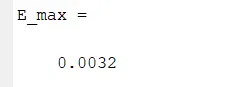
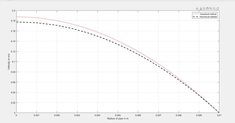
change in velocity along the radius of the pipe for both analytical and numerical method is shown in the below graph
both the velocity profiles are almost similar which validate the result