Week 7 - Simulation of a 1D Super-sonic nozzle flow simulation using Macormack Method
In this challenge you are going to simulate the isentropic flow through a quasi 1D subsonic-supersonic nozzle. You will derive both the conservation and non-conservation forms of the governing equations and sovle them using the MacCormack's technique. You need to determine the steady-state temperature distribution for the flow-field variables and investigate the difference between the two forms of governing equations by comparing their solutions.
You need to show the following plots inside your report
1. Steady-state distribution of primitive variables inside the nozzle
2. Time-wise variation of the primitive variables
3. Variation of Mass flow rate distribution inside the nozzle at different time steps during the time-marching process
4. Comparison of Normalized mass flow rate distributions of both forms
There are two methods to solve almost every CFD problem numerically by using conservative and non conservative equations. From theoretical and mathemmatical view both forms are equivalent and cann be
converted into one another.
CONNSERVVATIVE FORM :
Consider an infinitesimal smalll fluid element inside nozzle, and the fluuid moving through that elements ,such type of condition is conservative form and the equation obtained obbtained in such cases are called as called as conservativve form of governing equations.
NON CONSERVATION FORM :
Consider an infinitesimal small fluid element inside nozzle,the fluid same fluid element moving along streamline,such type of condition is non conservative form and the equation obtained in such cases are called as non conservative form of governing equation .
SCHEMATIC FOR SUBSONIC- SUPERSONIC NOZZLE FLOW :
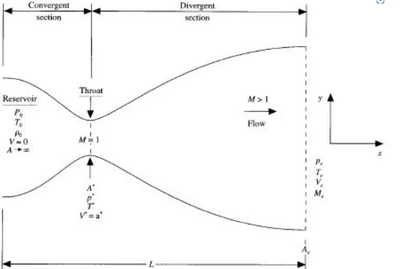
The above figure shows schematic diagram of convergent divergent nozzle.
The flow a inlet of nozzle come from reservoir .For the convergent section flow is subsonic MACH NUMBER <1,divergent section flow is supersonic MACH NUMBER>1 and at throaat flow is sonic
MACH NUMBER =1.
GOVERNING EQUATIONS :
As we considereing the flow through is only functionn of X and not Y ,hence we must apply integgral form of Navier-stokes equation to a control volume consistent with the quasi 1D assumption.Hence by referring below figure we obtain PDE form of governing equatiions from integral forms.
The shaded region is brlow figure shows control volume,slice of nozzle flow with infinitesimal thickness of dx.
CONTROL VOLUME FOR DERIVING THE PARTIAL DIFFERENTIAL EQUATIONS FOR UNSTEADY,QUASI ONE-DIMENSIONAL FLOW.
Since the problem is set up in 1D,We consider only distribution in the x-axis .Here Nozzle can be split into two sections
1.Convergent Section
2.Divergent Section
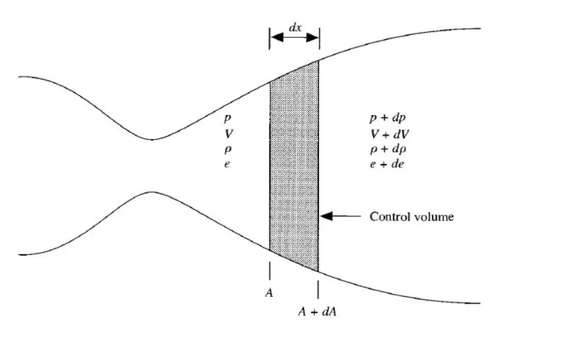
For the Quasi 1D flow governing equations are as follows -
-Continuity equation :
rho1*A1*V1 = rho2*A2*V2
-Momentum equationn :
P1*A1+rho1*A1*V1+integral_A1toA2 P*da = P2*A2+rho2*A2*V2^2
Energy equation -
h1+v1^2/2 = h2+V2^2/2
Where,
h = c_p*T
NOZZLE FLOW PROBLEM :
DISCRETIZATION :
It can be done by setting a finite difference expressions using macCormak's explicit technique.
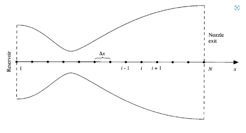
The PDE is discretized and sollved for the points in the dommain.The Maccormack method is used for discretizing the equation.The Maccormack method gives better resullts for the hyperbolic equation and it is called a shock -capturing method.These methods cann provide stable solution in the presence of shock.Hence they are used inn nozzle flow problems.In the Maccormack method commbination of both forward and backward differencing schemes can be used to solve foe the primitive variables Non-conservativve and conservative forms of govering equations are solved by using thhis method .
1.Initial condition
2.Boundary condition
Initial condition :
A = 1+2.2(x-1.5)^2 0<=x<=3
rho = 1-0.3146x
T = 1-0.2314x
V = (0.1+1.09x)T^1/2
Boundary Condition :
At point 1
rho_1 = 1
T_1 = 1
V_1 = 2V_2-V_3
At point n
V_n = 2V_n-1-V_n-2
rho_n = 2rho_n-1-rho_n-2
T_n = 2T_n-1-T_n-2
1. Non-Conservative form :
Predictor step : [forward differencing]]
Continuity equation :

Momentum equatiion :

Energy equation :

Now to obtain predicted values of
'rho','V','T'
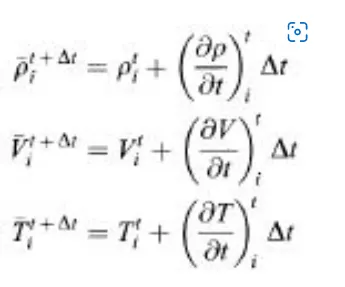
Corrector values :[Backward diffrencing] :
Continuity equation :
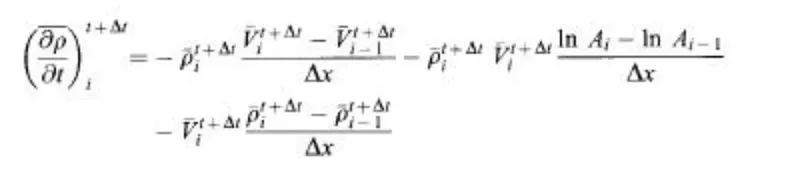
Momentum equation :

Energy equation :
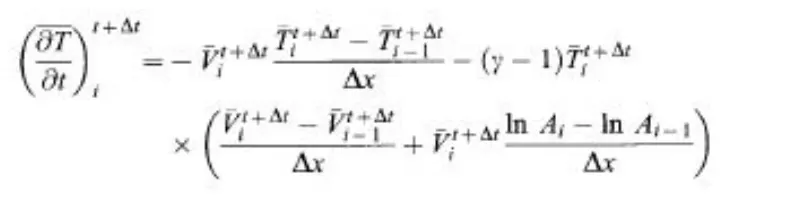
The average time derivative values can be calculaated by taking average of corrector time derivative and predictor time derivvative values as follows,
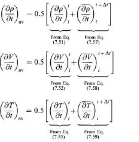
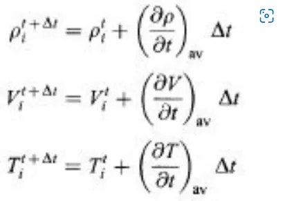
The final value of
'rho','V','T'
Can be obtained from followinng equations
Initial condition :
rho = 1-0.3146x
T = 1-0.2314x
V = (0.1+1.09x).T^1/2
Boundary conditions :
Conservative form :
F1 = F1(U1,U2,U3)
F2 = F2(U1,U2,U3)
F3 = F3(U1,U2,U3)
J2 = J(U1,U2,U3)
Predictor step :
dU1/dt = F1_(i+1) -F1_(i)/dx
dU2/dt = F2_(i+1)-F2(i)/dx + J2_(i+1)-J2_(i)/dx
dU3/dt = F3_(i+1)-F3(i)/dx
For corrector method updating values of U1,U2&U3.
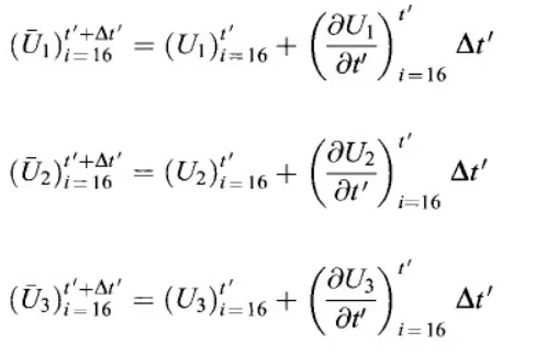
Corrector Step :
dU1/dt = F1_(i) -F1_(i-1)/dx
dU2/dt = F2_(i)-F2(i-1)/dx + J2_(i)-J2_(i-1)/dx
dU3/dt = F3_(i)-F3(i-1)/dx
The average time derivative values can be calculated by taking average of corrector time derivative and predictor time derivativve values as follows ,
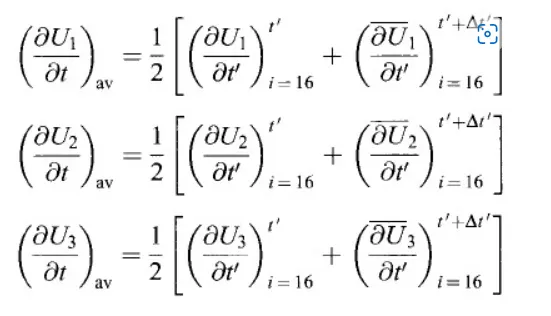
Hence the final values of U1,U2 &U3 are obtain from following equations.
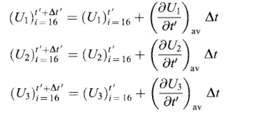
NON-DIMENSIONNAL QUANTITIES :
Also as part of the problem setup,we represent quantities in terms of non-dimensiional quantites .
Temperature T' = T/T_o
Density : rho' = rho/rho_o
Non dimensional distannce x' = x/L
Non - dimmensional velocity : V' = V/a_o where 'a_o' is the local sonic velocity (a_o = `sqrt(gammaRT_o)`
Non-dimensional Time t' = t/L/a_o where L/a_o is characteristic time scale
Non-dimensional area = A' = A/A*
The prime in the above equation representts thhe non-dimensional form of governing equation.The non-dimmensional form of the Navier stokkes equation can ease thhe analysis of the problem
and reduce the number of parameters.The difference between the conservative and non conservative form of governning equationn is that both forms pf governing equation is that both forms give the same
analytical solution but different numerical output.Conservattive form provides accurate results and it can provide better results in the presence of shockks or discontinuitities.
MACCORMACK METHOD :
To discretize the numerical solution,we use the technique called the MaccCormack method.The MacCormack method is a variation of the Teo-Step LAx-Wendroff Scheme but is much simpler in the
application.
The application of the MacCormack method proceeds in two steps,
A particular step Which is followed by a corrector step.
Steps involved in MacCormack method
1.predictor Step
2.Solution update
3.Corrector step
4.Determining the average of the time derivative
5.Final solution update
1.PREDICTOR STEP :
In the predictor step,a 'provisional' value of at time level is estimated obtained by replacing the spatial and temporal derivatioves in the previous first-order equation usinng the Forward differencing scheme.
It is used in Timestep.
2. CORRECTOR STEP :
In the corrector step,the predicted value is corrected according to the equation .Note that the corrector step uses the Backward differences schenme for spatial derivatives.The time-step used in the corrector
step is in conntrast to the used in the predictor step.
MATLAB CODE :
FUNCTION FOR NON-CONSERVATIVE FORM :
% Function for  Non conservation form

function [Mass_flow_rate_NC,Pressure_NC,Mach_number_NC,rho_NC,v_NC,T_NC,rho_throat_NC,v_throat_NC,T_throat_NC,Mass_flow_rate_throat_NC,Pressure_throat_NC,Mach_number_throat_NC] = Non_conservative_form(x,dx,n,gamma,nt,C)

% initial profiles
rho_NC = 1-0.3146*x;
T_NC = 1-0.2341*x;
v_NC = (0.1+1.09*x).*T_NC.^0.5;

% Area & Throat profiles
a = 1+2.2*(x-1.5).^2;
throat = find(a==1);

% outer time loop

for k = 1:nt

    % Time-step control
    dt = min(C.*dx./(sqrt(T_NC)+v_NC));

    %  saving old values
    rho_old = rho_NC;
    T_old = T_NC;
    v_old = v_NC;

    % predictor method

    for j = 2:n-1

        % simplifying the Equation's spatial forms
        dv_dx = (v_NC(j+1) - v_NC(j))/dx;
        drho_dx = (rho_NC(j+1) - rho_NC(j))/dx;
        dT_dx = (T_NC(j+1) - T_NC(j))/dx;
        dlog_a_dx = (log(a(j+1)) - log(a(j)))/dx;

        % continuity equation

        drho_dt_P(j) = -rho_NC(j)*dv_dx-rho_NC(j)*v_NC(j)*dlog_a_dx - v_NC(j)*drho_dx;

        % momentum equation
        dv_dt_P(j) = -v_NC(j)*dv_dx-(1/gamma)*(dT_dx+(T_NC(j)*drho_dx/rho_NC(j)));

        % energy equation
        dT_dt_P(j) = -v_NC(j)*dT_dx-(gamma-1)*T_NC(j)*(dv_dx+v_NC(j)*dlog_a_dx);


        % solution update
        rho_NC(j) = rho_NC(j) + drho_dt_P(j)*dt;
        v_NC(j) = v_NC(j) + dv_dt_P(j)*dt;
        T_NC(j) = T_NC(j) + dT_dt_P(j)*dt;

    end

    % corrector method

    for j = 2:n-1


        % simplifying the Equation's spatial forms
        dv_dx = (v_NC(j) - v_NC(j - 1))/dx;
        drho_dx = (rho_NC(j) - rho_NC(j - 1))/dx;
        dT_dx = (T_NC(j) - T_NC(j - 1))/dx;
        dlog_a_dx = (log(a(j)) - log(a(j-1)))/dx;

        % continuity equation

        drho_dt_C(j) = -rho_NC(j)*dv_dx - rho_NC(j)*v_NC(j)*dlog_a_dx - v_NC(j)*drho_dx;

        % momentum equation
        dv_dt_C(j) = -v_NC(j)*dv_dx - (1/gamma)*(dT_dx+(T_NC(j)*drho_dx/rho_NC(j)));

        % energy equation
        dT_dt_C(j) = -v_NC(j)*dT_dx - (gamma-1)*T_NC(j)*(dv_dx+v_NC(j)*dlog_a_dx);

    end

    % compute average time  derivative
    drho_dt = 0.5.*(drho_dt_P+drho_dt_C);
    dv_dt = 0.5.*(dv_dt_P+dv_dt_C);
    dT_dt = 0.5.*(dT_dt_P+dT_dt_C);

    % final solutionn update

    for i = 2:n-1
        rho_NC(i) = rho_old(i)+drho_dt(i)*dt;
        v_NC(i) = v_old(i)+dv_dt(i)*dt;
        T_NC(i) = T_old(i)+dT_dt(i)*dt;

    end

    % applying boundary conditions

    % AT inlet

    rho_NC(1) = 1;
    v_NC(1) = 2*v_NC(2)-v_NC(3);
    T_NC(1) = 1;

    % at outlet

    rho_NC(n) = 2*rho_NC(n-1)-rho_NC(n-2);
    v_NC(n) = 2*v_NC(n-1)-v_NC(n-2);
    T_NC(n) = 2*T_NC(n-1)-T_NC(n-2);

    % defining mass flow rate, pressure and mach number
    Mass_flow_rate_NC = rho_NC.*a.*v_NC;
    Pressure_NC = rho_NC.*T_NC;
    Mach_number_NC = (v_NC./sqrt(T_NC));

    % calculating variables at throat section

    rho_throat_NC(k) = rho_NC(throat);
    T_throat_NC(k) = T_NC(throat);
    v_throat_NC(k) = v_NC(throat);
    Mass_flow_rate_throat_NC(k) = Mass_flow_rate_NC(throat);
    Pressure_throat_NC(k) = Pressure_NC(throat);
    Mach_number_throat_NC(k) = Mach_number_NC(throat);

    % plotting

    % comparisionn of non-dimensional mass flow rates at different time
    % steps

    figure(1);
     if k == 50
         plot(x,Mass_flow_rate_NC,'m','linewidth',1.25)
         hold on
     elseif k == 100
         plot(x,Mass_flow_rate_NC,'c','linewidth',1.25)
         hold on
     elseif k == 200
         plot(x,Mass_flow_rate_NC,'g','linewidth',1.25)
         hold on
     elseif k == 400
         plot(x,Mass_flow_rate_NC,'y','linewidth',1.25)
         hold on
     elseif k == 800
         plot(x,Mass_flow_rate_NC,'k','linewidth',1.25)
         hold on
     end

     % label
     title('Mass flow rates at different Time-steps-NON CONSERVATIVE FORM')
     xlabel('Distance')
     ylabel('Mass flow rate')
     legend({'50^t^h Timestep','100^t^h Timestep',' 200^t^h Timestep','400^t^h Timestep','800^t^h Timestep'})
     axis([0 3 0 2])
     grid on
end
end
FUNCTION FOR CONSERVATIVE FORM :
% Function for conservative form

function [Mass_flow_rate_C,Pressure_C,Mach_number_C,rho_C,v_C,T_C,rho_throat_C,v_throat_C,T_throat_C,Mass_flow_rate_throat_C,Pressure_throat_C,Mach_number_throat_C] = Conservative_form(x,dx,n,gamma,nt,C)

% determing initial profile of density and temperatture

for i = 1:n

    if (x(i)>= 0 && x(i) <=0.5)
        rho_C(i) = 1;
        T_C(i) = 1;
    elseif (x(i) >= 0.5 && x(i) <= 1.5)
        rho_C(i) = 1- 0.366*(x(i)-0.5);
        T_C(i) = 1-0.167*(x(i)-0.5);
    elseif (x(i) >= 1.5 && x(i) <= 3)
        rho_C(i) = 0.634-0.3879*(x(i)-1.5);
        T_C(i) = 0.833-0.3507*(x(i)-1.5);

    end

end

% area and throat profiles
a = 1+2.2*(x-1.5).^2;
throat = find(a==1);

% initial profile for velocity  and pressure
v_C = 0.59./(rho_C.*a);
Pressure_C = rho_C.*T_C;

% calculate the initial solution vectors(U)
U1 = rho_C.*a;
U2 = rho_C.*a.*v_C;
U3 = rho_C.*a.*(T_C./(gamma-1)) + ((gamma/2).*v_C.^2);

% outer time loop
for  k = 1:nt

    % Time -step control
    dt = min(C.*dx./(sqrt(T_C)+v_C));

    % savinng old values
    U1_old = U1;
    U2_old = U2;
    U3_old = U3;

% calculatinng te flux vector (F)

F1 = U2;
F2 = ((U2.^2)./U1)+((gamma-1)/gamma)*(U3-(gamma/2)*((U2.^2)./U1));
F3 = ((gamma*U2.*U3)./U1)-(gamma*(gamma-1)*((U2.^3)./(2*U1.^2)));

% predictor method
for j = 2:n-1

    % calculating the source term(J)
    J2(j) = (1/gamma)*rho_C(j)*T_C(j)*((a(j+1)-a(j))/dx);

    % continuity equation
    dU1_dt_P(j) = -((F1(j+1)-F1(j))/dx);

    % momentum equation
    dU2_dt_P(j) = -((F2(j+1)-F2(j))/dx)+J2(j);

    % energy equati
    dU3_dt_P(j) = -((F3(j+1)-F3(j))/dx);

    % updating new values
    U1(j) = U1(j) + dU1_dt_P(j)*dt;
    U2(j) = U2(j) + dU2_dt_P(j)*dt;
    U3(j) = U3(j) + dU3_dt_P(j)*dt;

end

% updating flux vectors

F1 = U2;
F2 = ((U2.^2)./U1)+((gamma-1)/gamma)*(U3-((gamma*0.5*(U2.^2))./U1));
F3 = ((gamma*U2.*U3)./U1)-((gamma*0.5*(gamma-1)*(U2.^3))./(U1.^2));


% corrector method

for j = 2:n-1


 % calculating the source term(J)
    J2(j) = (1/gamma)*rho_C(j)*T_C(j)*((a(j)-a(j-1))/dx);

    % continuity equation
    dU1_dt_C(j) = -((F1(j)-F1(j-1))/dx);

    % momentum equation
    dU2_dt_C(j) = -((F2(j)-F2(j-1))/dx)+J2(j);

    % energy equation

     dU3_dt_C(j) = -((F3(j)-F3(j-1))/dx);

end

% compute average time derivative
dU1_dt = 0.5*(dU1_dt_P+dU1_dt_C);
dU2_dt = 0.5*(dU2_dt_P+dU2_dt_C);
dU3_dt  = 0.5*(dU3_dt_P+dU3_dt_C);

% finall solution update

for i = 2:n-1
    U1(i) = U1_old(i)+dU1_dt(i)*dt;
    U2(i) = U2_old(i)+dU2_dt(i)*dt;
    U3(i) = U3_old(i) +dU3_dt(i)*dt;

end

% applying boundary conditions

% at inlet
U1(1) = rho_C(1)*a(1);
U2(1) = 2*U2(2)-U2(3);

v_C(1) = U2(1)./U1(1);
U3(1) = U1(1)*((T_C(1)/(gamma-1))+((gamma/2)*(v_C(1)).^2));


% at outlet
U1(n) = 2*U1(n-1)-U1(n-2);
U2(n) = 2*U2(n-1)-U2(n-2);
U3(n) = 2*U3(n-1)-U3(n-2);


% final primitive value update

rho_C = U1./a;
v_C = U2./U1;
T_C = (gamma-1)*((U3./U1-(gamma/2)*(v_C).^2));


% defining mass flow rate ,Prsuure and mach number
Mass_flow_rate_C = rho_C.*a.*v_C;
Pressure_C = rho_C.*T_C;
Mach_number_C = (v_C./sqrt(T_C));


% calculating variables at throat section
rho_throat_C(k) = rho_C(throat);
T_throat_C(k) = T_C(throat);
v_throat_C(k) = v_C(throat);
Mass_flow_rate_throat_C(k) = Mass_flow_rate_C(throat);
Pressure_throat_C(k) = Pressure_C(throat);
Mach_number_throat_C(k) = Mach_number_C(throat);

% plotting

% comparision of non-dimensional mass flow rates at different time steps

figure(4)
if k == 50
    plot(x,Mass_flow_rate_C,'m','linewidth',1.25);
    hold on
elseif k == 100
    plot(x,Mass_flow_rate_C,'c','linewidth',1.25);
    hold on
elseif k == 200
    plot(x,Mass_flow_rate_C,'g','linewidth',1.25);
    hold on
elseif k == 400
    plot(x,Mass_flow_rate_C,'y','linewidth',1.25);
    hold on
elseif k == 800
    plot(x,Mass_flow_rate_C,'k','linewidth',1.25);
    hold on

end

% label
title('Mass flow rates at different Time-steps- CONSERVATIVE FORM')
     xlabel('Distance')
     ylabel('Mass flow rate')
     legend({'50^t^h Timestep','100^t^h Timestep',' 200^t^h Timestep','400^t^h Timestep','8006t^h Timestep'})
     axis([0 3 0.4 2])
     grid on

end

end
MAIN CODE :
% solving 1D supersonic nozzle flow
clear all
close all
clc


% inputs
 n = 31;  % no.of grid points
 gamma = 1.4;
 x = linspace(0,3,n);
 dx = x(2)-x(1);

 nt = 1400;  % no. of time steps

 C = 0.5;  % courant number


 tic ;  %Non conservative form function

[Mass_flow_rate_NC,Pressure_NC,Mach_number_NC,rho_NC,v_NC,T_NC,rho_throat_NC,v_throat_NC,T_throat_NC,Mass_flow_rate_throat_NC,Pressure_throat_NC,Mach_number_throat_NC] = Non_conservative_form(x,dx,n,gamma,nt,C);

Time_elapsed_NC = toc;
fprintf('Time elapsed for non conservative form : % 0.4f',Time_elapsed_NC);
hold on


figure(2)  % Timestep variation of properties at throat area in non conservative form
%Density
subplot(4,1,1)
plot(linspace(1,nt,nt),rho_throat_NC,'color','k')
ylabel('Density')
legend({'Density at throat'});
axis([0 1400 0 1.3]);
grid minor;
title('Timestep variation at throat area-NON CONSERVATIVE FORM')

% temperature
subplot(4,1,2)
plot(linspace(1,nt,nt),T_throat_NC,'color','r')
ylabel('Temperature')
legend({'Temperature at throat'});
axis([0 1400 0.6 1]);
grid on

%Pressure

subplot(4,1,3)
plot(linspace(1,nt,nt),Pressure_throat_NC,'color','C')
ylabel('Pressure')
legend({'Prssure at throat'});
axis([0 1400 0.4 1.1]);
grid on
% mach number
subplot(4,1,4)
plot(linspace(1,nt,nt),Mach_number_throat_NC,'color','m')
xlabel('Timesteps')
ylabel('Mach number')
legend({'Mach number at throat'});
axis([0 1400 0.6 1.4])
grid on

figure(3);   % steady state simulation for primitive vallues for non-conservative form
%density
subplot(4,1,1);
plot(x,rho_NC,'color','y')
ylabel('Density')
legend({'Density'})
axis([0 3 0 1])
grid minor;
title('Varaiatiion of floe rste Distributor-NON CONSERVATIVVE FORM')

% Temperature
subplot(4,1,2);
plot(x,T_NC,'color','c')
ylabel('Temperature')
legend({'Temperature'});
axis([0 3 0 1])
grid on

% Pressure
subplot(4,1,3);
plot(x,Pressure_NC,'color','g')
ylabel('Pressure')
legend({'Pressure'})
axis([0 3 0 1])
grid on

% mach number
subplot(4,1,4);
plot(x,Mach_number_NC,'color','y')
xlabel('Nozzle Length')
ylabel('mach number')
legend({'Mach number'});
axis([0 3 0 4])
grid on


tic; % conservative form
[Mass_flow_rate_C,Pressure_C,Mach_number_C,rho_C,v_C,T_C,rho_throat_C,v_throat_C,T_throat_C,Mass_flow_rate_throat_C,Pressure_throat_C,Mach_number_throat_C] = Conservative_form(x,dx,n,gamma,nt,C);
Time_elapsed_C = toc;
fprintf('Timme elasped for conservative form : % 0.4f',Time_elapsed_C);


figure(5)  % Timestep variation of properties at throat area in  conservative form
% Density
subplot(4,1,1)
plot(rho_throat_NC,'color','m')
ylabel('Density')
legend({'Density at throat'});
axis([0 1400 0 1]);
grid on
title('Timestep variation at throat area- CONSERVATIVE FORM')

% temperature
subplot(4,1,2)
plot(T_throat_NC,'color','c')
ylabel('Temperature')
legend({'Temperature at throat'});
axis([0 1400 0.6 1]);
grid on

% Pressure

subplot(4,1,3)
plot(Pressure_throat_NC,'color','C')
ylabel('Pressure')
legend({'Prssure at throat'});
axis([0 1400 0.2 0.8]);
grid on


% mach number
subplot(4,1,4)
plot(Mach_number_throat_NC,'color','y')
xlabel('Timesteps')
ylabel('Mach number')
legend({'Mach number at throat'});
axis([0 1400 0.6 1.4])
grid on

figure(6);   % steady state simulation for primitive vallues for conservative form
% density
subplot(4,1,1);
plot(x,rho_C,'color','m')
ylabel('Density')
legend({'Density'})
axis([0 3 0 1])
grid on
title('Varaiatiion of flow rste Distributor- CONSERVATIVVE FORM')

% Temperature
subplot(4,1,2);
plot(x,T_C,'color','c')
ylabel('Temperature')
legend({'Temperature'});
axis([0 3 0 1])
grid on

% Pressure
subplot(4,1,3);
plot(x,Pressure_C,'color','g')
ylabel('Pressure')
legend({'Pressure'})
axis([0 3 0 1])
grid on
% mach number
subplot(4,1,4);
plot(x,Mach_number_C,'color','y')
xlabel('Nozzle Length')
ylabel('mach number')
legend({'Mach number'});
axis([0 3 0 4])
grid on

figure(7) % comparision of normalized mass flow rate of both forms
hold on
plot(x,Mass_flow_rate_NC,'r','linewidth',1.25)
hold on
plot(x,Mass_flow_rate_C,'k','linewidth',1.25)
hold on
grid on
legend('Non Conservative','Conservative')
xlabel('length of the domain')
ylabel('Mass flow rate')
title('Comparison of normalized mass flow rate of both forms')
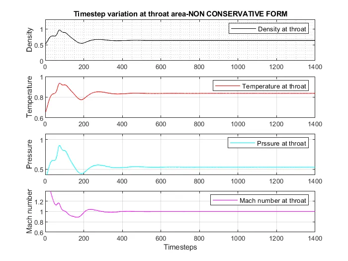
TIME STEPS VARIATION OF A PRIMMITATIVE VARIABBLE AT THROAT AREA :
NON-CONSERVATIVE FORM :
CONSERVATIVE FORM :
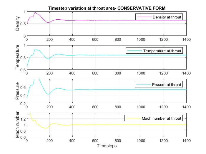
By observing the abovve plots we can conclude that initial variations observed in the Non-Conservative form form for a certain period make it conume a higher amount of time to achieve a stable solution when compared to the Conservative form.
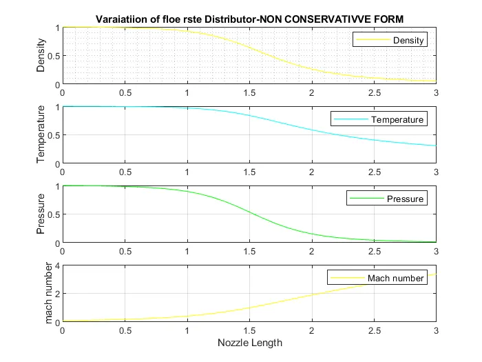
TIME MARCHING PROCESS :
NON-CONSERVATIVE FORM :
CONSERVATIVE FORM :
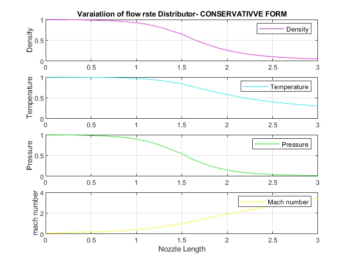
By observing the above plots we can conclude that we coudld see that both forms in the same phase giving the same solution for all the values.
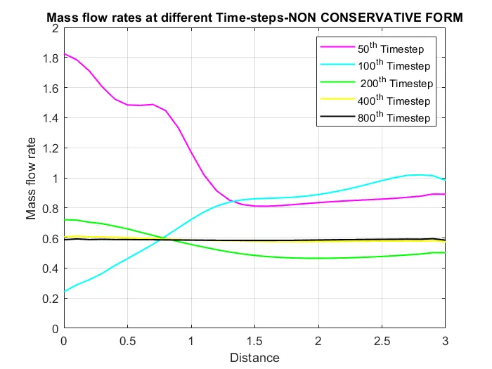
MASS FLOW RATE AT DIFFFERENT TIME SREPS :
NON-CONSERVATIVE FORM :
CONSERVATIVE FORM :
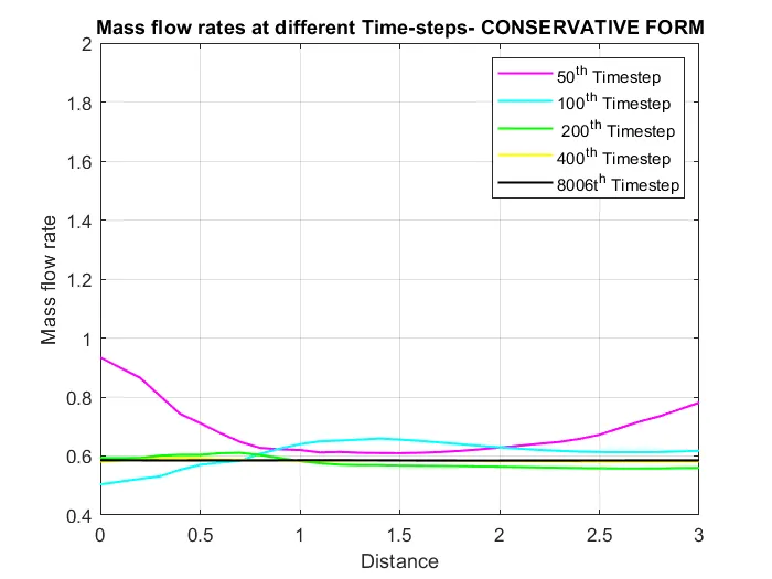
By observing the above plots we can conclude that mass flow rate at different time steps along the distance oscillates initially,however,the solution becomes stable after thhe 400th Time step for both the forms attaining a constant value.
COMPARISION OF NORMALIZED MASS FLOW RATE DISTRIBUTIONS OF BOTH FORMS :
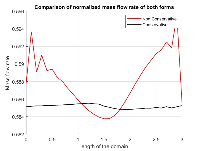
Both forms have their own merits and demerits and one should choose the form according to requirements.The non-consevative form produces accurate results for the primitive variabble and the conservative
form gives better results for the flux variable/vector.the cumulating that the above results we can conclude that the connservative form converges slightly
faster than the non-conservative from offering a stable solution along with the simulation .Yet both the forms are dependable inn calculating the almost precise solutions.