Week 7 - Simulation of a 1D Super-sonic nozzle flow simulation using Macormack Method
Aim :
To simulate the isentropic flow through a quasi 1D subsonic-supersonic nozzle. You will derive both the conservation and non-conservation forms of the governing equations and sovle them using the MacCormack's technique.
Solution :
Matlab Code for Super Sonic flow Simulation
close all
clear all
clc
% length of nozzle
L = 3;
% Number of grid points
n = [31 62 93];
% Number of time steps
nt = 1:1400;
% CFL number
cfl = 0.5;
for i = 1:length(n)
x = linspace(0,L,n(i));
[mfr_nc,mfr_throat_nc] = non_conservative(L,n(i),nt,cfl);
[mfr_c,mfr_throat_c] = conservative(L,n(i),nt,cfl);
figure(7)
subplot(2,1,1)
plot(nt,mfr_throat_c,'b',nt,mfr_throat_nc,'r','linewidth',1)
xlabel('Time steps (nt)')
ylabel('Mass flow rate')
legend('Conservative form','Non-Conservative form')
title('Mass flow rate using "Non-Conservative form Vs Conservative form" at throat point i=16')
subplot(2,1,2)
plot(x,mfr_c,'b',x,mfr_nc,'r','linewidth',1)
xlabel('Length of Nozzel')
ylabel('Mass flow rate')
legend('Conservative form','Non-Conservative form')
title('Mass flow rate using "Non-Conservative form Vs Conservative form" in the nozzel')
figure(8)
subplot(2,1,1)
plot(nt,mfr_throat_c,'linewidth',1)
hold on
xlabel('Time steps (nt)')
ylabel('Mass flow rate')
legend('@31 nodes','@62 nodes','@93 nodes')
title('Conservative form : Grid independency test at throat point i=16')
subplot(2,1,2)
plot(nt,mfr_throat_nc,'LineWidth',1)
hold on
xlabel('Time steps (nt)')
ylabel('Mass flow rate')
legend('@31 nodes','@62 nodes','@93 nodes')
title('Non-Conservative form : Grid independency test at throat point i=16')
figure(9)
subplot(2,1,1)
plot(x,mfr_c,'LineWidth',1)
hold on
xlabel('Length of Nozzel')
ylabel('Mass flow rate')
legend('@31 nodes','@62 nodes','@93 nodes')
title('Conservative form : Grid independency test along the nozzle')
subplot(2,1,2)
plot(x,mfr_nc,'LineWidth',1)
hold on
xlabel('Length of Nozzel')
ylabel('Mass flow rate')
legend('@31 nodes','@62 nodes','@93 nodes')
title('Non-Conservative form : Grid independency test along the nozzle')
end
Conservative Function :
Matlab code for the Conservativce function
function [mfr_c,mfr_throat_c] = conservative(L,n,nt,cfl)
x = linspace(0,L,n);
dx = x(2)-x(1);
% Initial conditions rho,a,v,T,M,mfr,p
for ii = 1:length(x)
if (x(ii)<=0.5)
rho(ii) = 1;
T(ii) = 1;
elseif (x(ii)>0.5) & (x(ii)<=1.5)
rho(ii) = 1-0.366*(x(ii)-0.5);
T(ii) = 1-0.167*(x(ii)-1.5);
elseif (x(ii)>1.5) & (x(ii)<=3.5)
rho(ii) = 0.634-0.3879*(x(ii)-1.5);
T(ii) = 0.833-0.3507*(x(ii)-1.5);
end
end
% Area
a = 1 + 2.2*(x-1.5).^2;
% Gamma value
g = 1.4;
% Solution vectors u1, u2, u3
u1 = rho.*a;
u2 = 0.59*ones(1,n);
v = u2./u1;
u3 = u1.*((T./(g-1)) + (g/2).*v.^2);
% Mach Number
M = v./(T.^0.5);
% Mass flow rate
mfr = rho.*a.*v;
% Pressure
p = rho.*T;
% To find dt value
for z = 1:31
u = (T(z))^(1/2);
dt(z) = cfl*dx/(u + v(z));
end
dt = min(dt);
for i = 1:length(nt)
% To find dt value
for z = 1:31
u = (T(z))^(1/2);
dt(z) = cfl*dx/(u + v(z));
end
dt = min(dt);
% Storing Initial Values
u1_old = u1;
u2_old = u2;
u3_old = u3;
for j = 2:n-1
% Flux vectors
f1 = u2;
f2 = ((u2.^2)./u1) + ((g-1)/g) * (u3 - ((g/2)*(u2.^2)./u1));
f3 = ((g.*u2.*u3)./u1) - ((g*(g-1)/2) * (u2.^3)./(u1.^2));
% Source term
j1 = (1/g)*rho(j)*T(j)*((a(j+1) - a(j))/dx);
% Predictor step
% Continuity
du1_dt_p(j) = -(f1(j+1) - f1(j))/dx;
% Momentum
du2_dt_p(j) = -(f2(j+1) - f2(j))/dx + j1;
% Energy
du3_dt_p(j) = -(f3(j+1) - f3(j))/dx;
% Updating solution vectors
u1(j) = u1_old(j) + du1_dt_p(j)*dt;
u2(j) = u2_old(j) + du2_dt_p(j)*dt;
u3(j) = u3_old(j) + du3_dt_p(j)*dt;
end
% Updating Primitives
rho = u1./a;
T = (g-1).*(u3./u1-(g/2).*(u2./u1).^2);
for j = 2:(n-1)
% Source term for corrective step
j2 = (1/g)*(rho(j)*T(j)*(a(j)-a(j-1))/dx);
% Corrective step
% Continuity
du1_dt_c(j) = -(f1(j)-f1(j-1))/dx;
% Momentum
du2_dt_c(j) = j2-(f2(j)-f2(j-1))/dx;
% Energy
du3_dt_c(j) = -(f3(j)-f3(j-1))/dx;
end
% Average time derivatives
du1_dt_avg = 0.5*(du1_dt_p + du1_dt_c);
du2_dt_avg = 0.5*(du2_dt_p + du2_dt_c);
du3_dt_avg = 0.5*(du3_dt_p + du3_dt_c);
% Final corrected values
for k = 2:n-1
u1(k) = u1_old(k) + du1_dt_avg(k)*dt;
u2(k) = u2_old(k) + du2_dt_avg(k)*dt;
u3(k) = u3_old(k) + du3_dt_avg(k)*dt;
end
% Entry Boundary conditions
u1(1) = a(1);
u2(1) = 2*u2(2)-u2(3);
u3(1) = u1(1)*(T(1)/(g-1) + (g*(u2(1)/u1(1))^2/2));
% Exit Boundary conditions
u1(n) = 2*u1(n-1)-u1(n-2);
u2(n) = 2*u2(n-1)-u2(n-2);
u3(n) = 2*u3(n-1)-u3(n-2);
% Final update of primitives
rho = u1./a;
v = u2./u1;
T = (g-1).*(u3./u1-(g/2).*(u2./u1).^2);
p = rho.*T;
M = v./T.^0.5;
error(k) = abs(v(k) - v(k-1));
mfr = u2;
% To Find value at throat points
T_throat(i) = T(16);
rho_throat(i) = rho(16);
v_throat(i) = v(16);
M_throat(i) = M(16);
p_throat(i) = p(16);
error_throat(i) = error(16);
mfr_throat(i) = mfr(16);
if n == 31
for ii = [1:50:201 700]
if ii == i
figure (4)
plot(x,mfr,'LineWidth',1)
hold on
title('Non-conservative form - Variation of Mass flow rate distribution inside the nozzle at different time steps during the time marching process')
xlabel('Length of nozzle')
ylabel('Mass flow rate')
elseif i == 1400
plot(x,mfr,'*r')
legend('@1','@51','@101','@151','@201','@700','@1400')
end
end
end
mfr_c = mfr;
mfr_throat_c = mfr_throat;
end
figure(5)
plot(x,v,'b',x,p,'r',x,T,'k',x,rho,'m',x,M,'g',x,mfr,'c')
ylim([-0.1 3.7])
title(sprintf('Time step = %d',i))
xlabel('Length of nozzle')
ylabel('Non dimensional parameters')
legend('Velocity','Pressure','Temperature','Density','Mach Number','Mass flow rate','location','northwest')
title('Non-conservative form -Steady state distribution of primitive variables inside the nozzle')
figure(6)
plot(nt,rho_throat)
hold on
plot(nt,v_throat,'linewidth',1)
plot(nt,p_throat,'linewidth',1)
plot(nt,T_throat,'linewidth',1)
plot(nt,M_throat,'lineWidth',1)
plot(nt,mfr_throat,'linewidth',1)
xlabel('Time steps (nt)')
ylabel('Non dimensional parameters')
legend('Density','Velocity','Pressure','Temperature','Mach Number','Mass flow rate')
title('Non-conservative form - Time wise variation of the primitive variables at throat point i = 16')
Non-conservative Function :
Matlab code for Non-conservative function
function [mfr_nc,mfr_throat_nc] = non_conservative(L,n,nt,cfl)
x = linspace(0,L,n);
dx = x(2)-x(1);
% Initial conditions rho,a,v,T,mfr,M,p
rho = 1-0.3146*x;
T = 1-0.2314*x;
v = (0.1 + 1.09*x).*T.^0.5;
a = 1 + 2.2*(x-1.5).^2;
M = v./(T.^0.5);
mfr = rho.*a.*v;
p = rho.*T;
g = 1.4;
for z = 1:31
u = (T(z))^(1/2);
dt(z) = cfl*dx/(u + v(z));
end
dt = min(dt);
for i = 1:length(nt)
% Storing initial values
rho_old = rho;
T_old = T;
v_old = v;
for j = 2:n-1
% Predictor step
drho_dx = (rho(j+1) - rho(j))/dx;
dv_dx = (v(j+1) - v(j))/dx;
dT_dx = (T(j+1) - T(j))/dx;
da_dx = (log(a(j+1)) - log(a(j)))/dx;
% Continuity
drho_dt_p(j) = -rho(j)*dv_dx - rho(j)*v(j)*da_dx - v(j)*drho_dx;
% Momentum
dv_dt_p(j) = -v(j)*dv_dx - (1/g)*(dT_dx + (T(j)/rho(j))*drho_dx);
% Energy
dT_dt_p(j) = -v(j)*dT_dx - (g-1)*T(j)*(dv_dx + v(j)*da_dx);
% Updating primitives
v(j) = v_old(j) + dv_dt_p(j)*dt;
rho(j) = rho_old(j) + drho_dt_p(j)*dt;
T(j) = T_old(j) + dT_dt_p(j)*dt;
% Corrector Step
drho_dx = (rho(j) - rho(j-1))/dx;
dv_dx= (v(j) - v(j-1))/dx;
dT_dx = (T(j) - T(j-1))/dx;
da_dx = (log(a(j)) - log(a(j-1)))/dx;
% Continuity
drho_dt_c(j) = -rho(j)*dv_dx - rho(j)*v(j)*da_dx - v(j)*drho_dx;
% Momentum
dv_dt_c(j) = -v(j)*dv_dx - (1/g)*(dT_dx + (T(j)/rho(j))*drho_dx);
% Energy
dT_dt_c(j) = -v(j)*dT_dx - (g-1)*T(j)*(dv_dx + v(j)*da_dx);
end
% Average time derivatives
drho_dt_avg = 0.5*(drho_dt_p + drho_dt_c);
dv_dt_avg = 0.5*(dv_dt_p + dv_dt_c);
dT_dt_avg = 0.5*(dT_dt_p + dT_dt_c);
% Final corrected values
for k = 2:n-1
rho(k) = rho_old(k) + drho_dt_avg(k)*dt;
v(k) = v_old(k) + dv_dt_avg(k)*dt;
T(k) = T_old(k) + dT_dt_avg(k)*dt;
end
% Entry Boundary conditions
v(1) = 2*v(2) - v(3);
% Exit boundary conditions
v(n) = 2*v(n-1) - v(n-2);
rho(n) = 2*rho(n-1) - rho(n-2);
T(n) = 2*T(n-1) - T(n-2);
% Final update of Primitives
p = rho.*T;
M = v./T.^0.5;
error(k) = abs(v(k) - v(k-1));
mfr = rho.*a.*v;
% To find the values at throat point
T_throat(i) = T(16);
rho_throat(i) = rho(16);
v_throat(i) = v(16);
M_throat(i) = M(16);
p_throat(i) = p(16);
error_throat(i) = error(16);
mfr_throat(i) = mfr(16);
if n == 31
for ii = [1:50:201 700]
if ii == i
figure (1)
plot(x,mfr,'LineWidth',1)
hold on
title('Non-conservative form - Variation of Mass flow rate distribution inside the nozzle at different time steps during the time marching process')
xlabel('Length of nozzle')
ylabel('Mass flow rate')
elseif i == 1400
plot(x,mfr,'*r')
legend('@1','@51','@101','@151','@201','@700','@1400')
end
end
end
end
figure(2)
plot(x,v,'b',x,p,'r',x,T,'k',x,rho,'m',x,M,'g',x,mfr,'c')
ylim([-0.1 3.7])
title(sprintf('Time step = %d',i))
xlabel('Length of nozzle')
ylabel('Non dimensional parameters')
legend('Velocity','Pressure','Temperature','Density','Mach Number','Mass flow rate','location','northwest')
title('Non-conservative form -Steady state distribution of primitive variables inside the nozzle')
figure(3)
plot(nt,rho_throat)
hold on
plot(nt,v_throat,'linewidth',1)
plot(nt,p_throat,'linewidth',1)
plot(nt,T_throat,'linewidth',1)
plot(nt,M_throat,'lineWidth',1)
plot(nt,mfr_throat,'linewidth',1)
xlabel('Time steps (nt)')
ylabel('Non dimensional parameters')
legend('Density','Velocity','Pressure','Temperature','Mach Number','Mass flow rate')
title('Non-conservative form - Time wise variation of the primitive variables at throat point i = 16')
mfr_nc = mfr;
mfr_throat_nc = mfr_throat;
end
Output :
Figure (1)
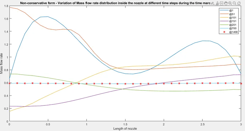
Figure (2) :
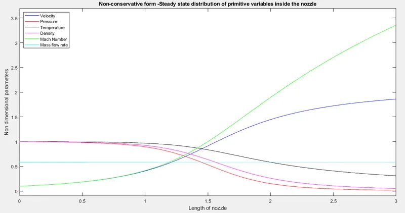
Figure (3)
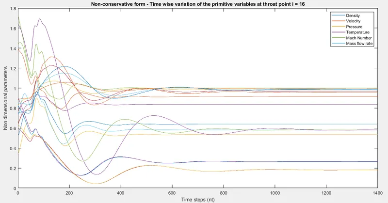
Figure (4)
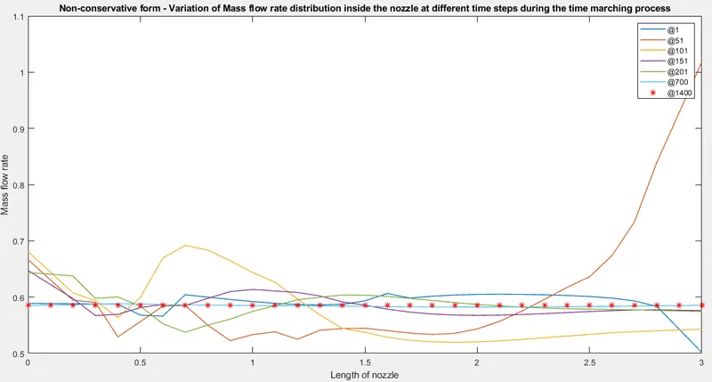
Figure (5)
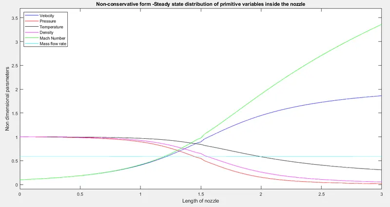
Figure (6)
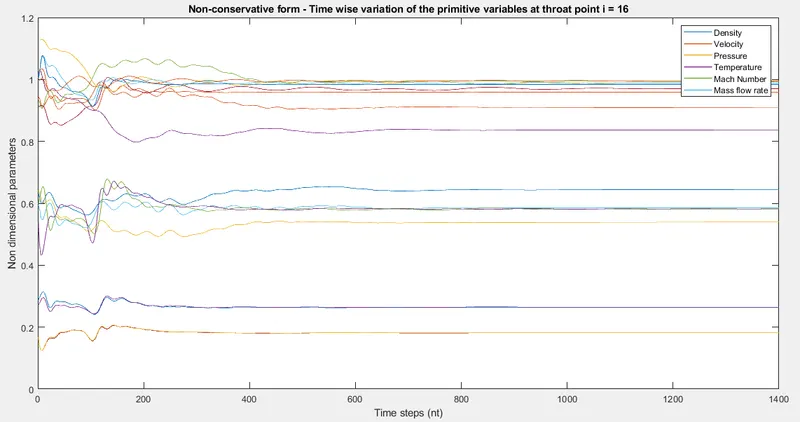
Figure (7)
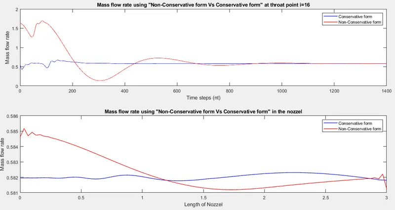
Figure (8)
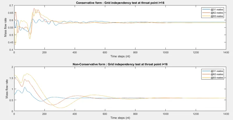
Figure (9)
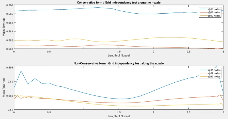
Figure (1) shows the steady state distribution of non-dimensional prmitive variables at end of the step.
Figure(2) shows the Time wise variation at the Primitive variables at the throat point i=16.
Figure(3) shows the variation of the Mass flow rate distribution inside the Nozzle at different time steps during the marching process.
Figure (7), (8) and (9) shows the various comparions between Conservative and Non-consrvative form.