Week 3.5 - Deriving 4th order approximation of a 2nd order derivative using Taylor Table method

AIM:

To find out the fourth order approximation of a 2nd order derivative using Taylor Table method. We will use the following methods to find out the fourth order approximation.

1. Central difference
2. Skewed right-sided difference
3. Skewed left-sided difference

CENTRAL DIFFERENCING SCHEMES:

No. of Nodes:

The number of nodes = p + q - 1

Where, p is the order of derivative and q is the order of approximations

The number of nodes = 2 + 4 - 1 = 5

Derivation:

To drive the fourth order approximation we start with this equation:

`del^2 u -: del x ^2 = a f (i - 2) + b f (i - 1) + c f(i) + d f (i + 1) + e f (i + 2) -: d x^2 .......(1)`

Taylor series derivation for the above terms :

`a f (i - 2) = a f(i) - 2af^'(i) dx -: 1! + 4 a f^'' (i) dx^2 -: 2! + 8 a f^''' (i) dx^3 -: 3! + 16 a f^'''' (i) dx^4 -: 4!`

Now, we write the terms from equation 1 in Taylor table form:

`dx^2 f ^''(i)`	`f(i)`	`f^'(i) dx`	`f^''(i) dx^2`	`f^'''(i) dx^3`	`f^''''(i) dx^4`
`af(i - 2)`	a	-2a	2a	`-4a // 3`	`2a // 3`
`bf(i - 1)`	b	-b	`b/2`	`-b / 6`	`b / 24`
`cf(i)`	c	0	0	0	0
`df (i + 1)`	d	d	`d // 2`	`d // 6`	`d // 24`
`e f (i +2)`	e	2e	2e	`4e // 3`	`2e // 3`
Sum of Co - efficients	0	0	1	0	0

the linear equation obtained from the above table is solved using matrix inversion method:

A.X = B

`[ [1 ,1, 1, 1, 1 ],[-2, -1, 0, 1, 2],[2, 1/2, 0, 1/2, 2],[-4/3, -1/6, 0, 1/6, 4/3],[2/3, 1/24, 0, 1/24, 2/3]]` . `((a),(b),(c),(d),(e))` = `((0),(0),(1),(0),(0))`

X = Inv(A)*B

we get the following results,

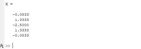
a = -0.0833, b = 1.3333, c = -2.5, d = 1.3333, e = -0.0833

SKEWED RIGHT HAND DIFFERENCE SCHEME:

NO. OF NODES:

The number of nodes = p + q

Where, P is the order of derivative and q is the order of approximations

The no. of nodes = 2 + 4 = 6

DERIVATION:

We us the following equation to find out the fourth order approximations,

`del u^2 -: del x^2 = a f(i) + b f (i +1) + c f (i + 2) + d f (i + 3) + e f(i + 4) + g f(i + 5) -: d x^2.......(2)`

Expanding all the terms and write it down in Taylor table form:

dx^2 f ^''(i)	f(i)	f^'(i) dx`	f^''(i)dx^2`	f^'''(i)dx^3`	f^''''(i)dx^4`	f^’’’’’(i)dx^5
af(i)	a	0	0	`0`	`0`	0
bf(i + 1)	b	b	`b/2`	`b /6`	`b /24`	b/120
cf(i + 2)	c	2c	4c/2	8c/6	16c/24	32c/120
df (i + 3)	d	3d	`9d/2`	27d/6`	81d/24`	243d/120
e f (i + 4)	e	4e	16e/2	64e/6`	256e/24	1024e/120
gf(i + 5)	g	5g	25g/2	125g/6	625g/24	3125g/120
Sum of Co-efficients	0	0	1	0	0	0

The above equation will be solved by matrix inversion method;

A.X = B

`[[1,1,1,1,1,1],[0,1,2,3,4,5],[0,1/2,4/2,9/2,16/2,25/2],[0,1/6,8/6,27/6,64/6,125/6],[0,1/24,16/24,81/24,256/24,625/24],[0,1/120,32/120,243/120,1024/120,3125/120]]`. `((a),(b),(c),(d),(e),(g))` = `((0),(0),(1),(0),(0),(0))`

X = inv(A)*B

By solving this we get the following results:

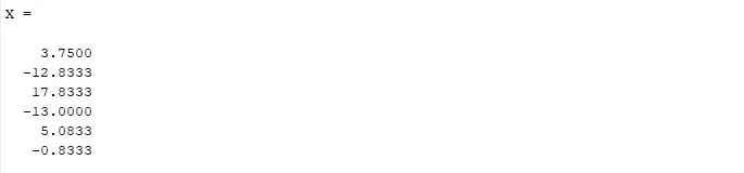
a = 3.75, b = -12.8333, c = 17.8333, d = -13, e = 5.0833, g = -0.8333

SKEWED LEFT HAND DIFFERENCE SCHEME:

No. of Nodes:

The number of nodes = p + q

Where, P is the order of derivative and q is the order of approximations

The no. of nodes = 2 + 4 = 6

DERIVATION:

To derive the fourth order approximation, we need to use the following equation:

`del^2 u / del x^2 = af(i - 5) + bf(i - 4) + cf(i - 3) + df(i - 2) + ef(i - 1) + gf(i) -: dx^2.....(3)`

expanding all the terms in the above equation gives us:

dx^2 f ^''(i)`	`f(i)`	f^'(i) dx`	f^''(i)dx^2`	f^'''(i) dx^3`	f^''''(i) dx^4`	f^’’’’’(i)dx^5
af(i - 5)`	a	-5a	25a/2	-125a/6`	625a/24	-3125a/120
`bf(i - 4)`	b	-4b	16b/2`	-64b/6	256b /24`	-1024b/120
cf(i - 3)`	c	-3c	9c/2	-27c/6	81c/24	-243c/120
`df (i - 2)`	d	-2d	4d/2`	-8d/6`	16d/24`	-32d/120
`e f (i - 1)`	e	-e	e/2	-e/6`	e/24	-e/120
gf(i)	g	0	0	0	0	0
Sum of Co-efficients	0	0	1	0	0	0

The linear equation will be solved by the matrix inversion method:

`[[1,1,1,1,1,1],[-5,-4,-3,-2,-1,0],[25/2,16/2,9/2,4/2,1/2,0],[-125/6,-64/6,-27/6,-8/6,-1/6,0],[625/24,256/24,81/24,16/24,1/24,0],[-3125/120,-1024/120,-243/120,-32/120,-1/120,0]]` * `((a``((a),(b),(c),(d),(e),(g))` = `((0),(0),(1),(0),(0),(0))`

X = inv(A)*B

By solving the following equation we get:

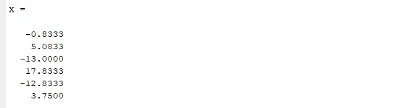
a = -0.8333, b = 5.0833, c = -13.0000, d = 17.8333, e = -12.8333, g = 3.7500

MATLAB CODE:

clear all
close all
clc

% Value of x
x = pi/3;

% range of dx
dx = linspace(pi/4,pi/4000,20);

for i = 1:length(dx)
    
    central_differencing(i) = fourth_order_central_differencing(x,dx(i));

    right_sided_skew(i) = fourth_order_right_sided_skew(x,dx(i));

    left_sided_skew(i) = fourth_order_left_sided_skew(x,dx(i));

end

% plotting
figure(1)
loglog(dx,central_differencing,'g')
hold on
loglog(dx,right_sided_skew,'b')
hold on
loglog(dx,left_sided_skew,'r')
xlabel('range of dx')
ylabel('truncation error')
legend('Central Differencing','Right handed skew','Left handed skew')

FUNCTION FOR CENTRAL DIFFERENCING:

function error_central_differencing = fourth_order_central_differencing(x,dx)

% Analytical function = exp(x)*cos(x);

% analytical_derivative
% f''(x) = -2*exp(x)*sin(x);

analytical_derivative = -2*exp(x)*sin(x);

% Numerical derivative

% central_differencing
central_differencing = (((-0.08333333*((exp(x-(2*dx)))*(cos(x-(2*dx)))))) + ((1.33333333)*((exp(x-dx))*(cos(x-dx)))) - ((2.5000)*((exp(x))*(cos(x)))) + ((1.33333333)*((exp(x+dx))*(cos(x+dx)))) - ((0.83333333)*((exp(x+(2*dx)))*(cos(x+(2*dx)))))) / (dx^2); 

% error
error_central_differencing = abs(central_differencing - analytical_derivative);

end

FUNCTION FOR RIGHT HANDED SKEW:

function error_right_sided_skew = fourth_order_right_sided_skew(x,dx)

% Analytical function = exp(x)*cos(x);

% analytical_derivative
% f''(x) = -2*exp(x)*sin(x);

analytical_derivative = -2*exp(x)*sin(x);

% Numerical derivative

% central_differencing
right_sided_skew = (((3.75)*((exp(x))*(cos(x))))) - ((12.83333333)*((exp(x+dx))*(cos(x+dx)))) + ((17.83333333)*((exp(x+(2*dx)))*(cos(x+(2*dx))))) - ((13.0000)*((exp(x+(3*dx)))*(cos(x+(3*dx))))) + ((5.08333333)*((exp(x+(4*dx)))*(cos(x+(4*dx))))) - ((0.83333333)*((exp(x+(5*dx)))*(cos(x+(5*dx))))) / (dx^2);

% error
error_right_sided_skew = abs(right_sided_skew - analytical_derivative);

end

FUNCTION FOR LEFT HANDED SKEW:

function error_left_sided_skew = fourth_order_left_sided_skew(x,dx)

% Analytical function = exp(x)*cos(x);

% analytical_derivative
% f''(x) = -2*exp(x)*sin(x);

analytical_derivative = -2*exp(x)*sin(x);

% Numerical derivative

% central_differencing
left_sided_skew = (((-0.8333)*((exp(x-(5*dx)))*(cos(x-(5*dx))))) + ((5.0833)*((exp(x-(4*dx)))*(cos(x-(4*dx))))) - ((13.0000)*((exp(x-(3*dx)))*(cos(x-(3*dx))))) + ((17.8333)*((exp(x-(2*dx)))*(cos(x-(2*dx))))) - ((12.8333)*((exp(x-dx)))*(cos(x-dx)))) + ((3.75)*((exp(x))*(cos(x)))) / (dx^2);

% error
error_left_sided_skew = abs(left_sided_skew - analytical_derivative);

end

CONCLUSION:

As seen from the graph the central differencing scheme has less error compared to other schemes. Therefore, central differencing is better than other schemes. As we see that central differencing uses data from both the sides and other schemes uses data from one side only.

WHY SKEWED SCHEME IS BETTER:

In some cases where we need to use the data from one side hence, we use skewed scheme instead of central differencing scheme.