Week 4.1 - Genetic Algorithm

clear all
close all
clc

% Defining our search space
x = linspace(0,0.6,150);
y = linspace(0,0.6,150);

num_spaces = 50;

% Creating a 2Dimensional Mesh
[xx, yy] = meshgrid(x, y);

% evaluating the stalagmite function
for i = 1:length(xx)
    for j = 1:length(yy)
        input_vector(1)=xx(i,j);
        input_vector(2)=yy(i,j);
        f(i,j) = stalagmite(input_vector);
    end
end


% study 1 = unbounded
tic
for i = 1:num_spaces 
    [results,fopt(i)] = ga(@stalagmite,2)
    xopt(i) = results(1)
    yopt(i) = results(2)
end

study_time1 = toc
figure(1)
subplot(2,1,1)
surf(x,y,-f)
shading interp
hold on
plot3 (xopt,yopt,-fopt,'marker','o','markersize',5,'markerfacecolor','r')
title('unbounded inputs')
subplot(2,1,2)
plot(-fopt)
xlabel('iteration')
ylabel('function maximum')

% study 2 = bounded
tic
for i = 1:num_spaces
    [results,fopt(i)] = ga(@stalagmite,2,[],[],[],[],[0;0],[0.6;0.6])
    xopt(i) = results(1)
    yopt(i) = results(2)
end

study_time2 = toc
figure(2)
subplot(2,1,1)
surf(x,y,-f)
shading interp
hold on
plot3 (xopt,yopt,-fopt,'marker','o','markersize',5,'markerfacecolor','r')
title('unbounded inputs')
subplot(2,1,2)
plot(-fopt)
xlabel('iteration')
ylabel('function maximum')

% study 3 = increased GA iterations
tic
options = optimoptions('ga');
options = optimoptions(options,'PopulationSize',200);
for i = 1:num_spaces
    [results,fopt(i)] = ga(@stalagmite,2,[],[],[],[],[0;0],[0.6;0.6],[],[],options)
    xopt(i) = results(1)
    yopt(i) = results(2)
end

study_time3 = toc
figure(3)
subplot(2,1,1)
surf(x,y,-f)
shading interp
hold on
plot3 (xopt,yopt,-fopt,'marker','o','markersize',5,'markerfacecolor','r')
title('unbounded inputs')
subplot(2,1,2)
plot(-fopt)
xlabel('iteration')
ylabel('function maximum')

The above program has been written to understand the genetic algorithm in Matalb using the stalgmite function.

Genetic Algorithms are search based algorithms based on natural selection and genetics. It is a subset of much larger branch known as Evolutionary Computation.

Program explanation:

clear all
close all
clc

% Defining our search space
x = linspace(0,0.6,150);
y = linspace(0,0.6,150);

num_spaces = 50;

Here, we are defining the values of X and y as 150 betwenn the intervals of 0 and 0.6.

Also we define the iterations to be 50

% Creating a 2Dimensional Mesh
[xx, yy] = meshgrid(x, y);

% evaluating the stalagmite function
for i = 1:length(xx)
for j = 1:length(yy)
input_vector(1)=xx(i,j);
input_vector(2)=yy(i,j);
f(i,j) = stalagmite(input_vector);
end

Since we need a 3D surface we create a 2D array of X and Y using meshgrid command and storing them in input_vector. We use this to call the Stalagmite Function.

function [A] = stalagmite (input_vector)
x = input_vector(1);
y = input_vector(2);
f1 = (sin(5.1*pi*x + 0.5))^6;
f2 = exp(-4*log(2)* (x - 0.0667)^2/0.64);
f3 = (sin(5.1*pi*y + 0.5))^6;
f4 = exp(-4*log(2)* (y - 0.0667)^2/0.64);

A = -f1*f2*f3*f4;
end

The above function is the Stalagmite function. We write this to get the output as -f so that in ga we get the maxima.

Now, we perform the first study,

% study 1 = unbounded
tic
for i = 1:num_spaces
[results,fopt(i)] = ga(@stalagmite,2)
xopt(i) = results(1)
yopt(i) = results(2)
end

study_time1 = toc
figure(1)
subplot(2,1,1)
surf(x,y,-f)
shading interp
hold on
plot3 (xopt,yopt,-fopt,'marker','o','markersize',5,'markerfacecolor','r')
title('unbounded inputs')
subplot(2,1,2)
plot(-fopt)
xlabel('iteration')
ylabel('function maximum')

We use plot3 to store the xopt and yopt and -fopt to get the optimum maxima. Also fopt is used to visualize iterations at a given time interval. Using tic and toc command we record the time taken to run the program.

The below plot generated :

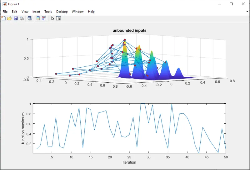
As we see in the above graph, we cant find the optimum values as they have gone outside the X and Y values.

Now, we perform 2nd Study,

% study 2 = bounded
tic
for i = 1:num_spaces
[results,fopt(i)] = ga(@stalagmite,2,[],[],[],[],[0;0],[0.6;0.6])
xopt(i) = results(1)
yopt(i) = results(2)
end

study_time2 = toc
figure(2)
subplot(2,1,1)
surf(x,y,-f)
shading interp
hold on
plot3 (xopt,yopt,-fopt,'marker','o','markersize',5,'markerfacecolor','r')
title('unbounded inputs')
subplot(2,1,2)
plot(-fopt)
xlabel('iteration')
ylabel('function maximum')

In the following study we define the lower and upper bound values.

We use plot3 to store the xopt and yopt and -fopt to get the optimum maxima. Also fopt is used to visualize iterations at a given time interval. Using tic and toc command we record the time taken to run the program.

The below plot generated :

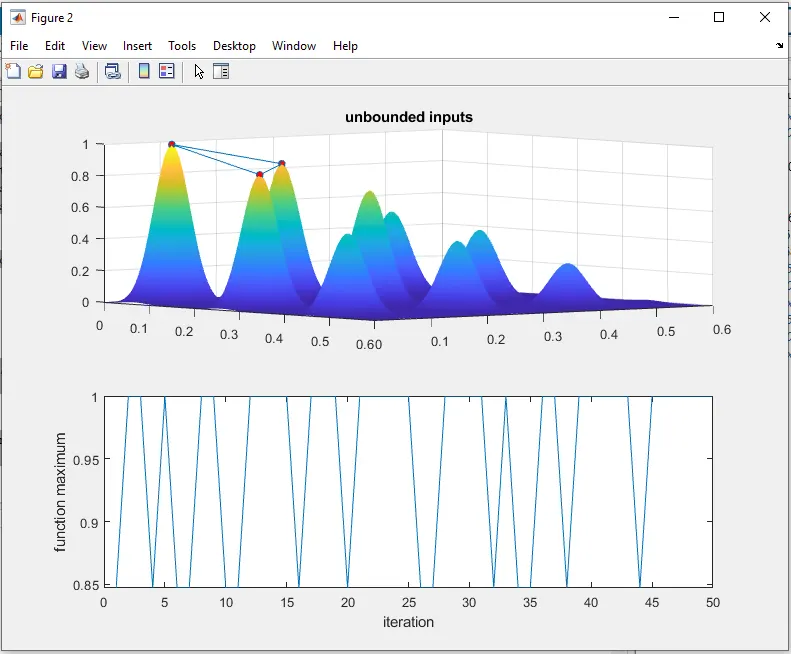
As we see in the following plot the optimum values are in the limit yet we cant find the exact values.

Hence, we perform the Study 3 :

% study 3 = increased GA iterations
tic
options = optimoptions('ga');
options = optimoptions(options,'PopulationSize',200);
for i = 1:num_spaces
[results,fopt(i)] = ga(@stalagmite,2,[],[],[],[],[0;0],[0.6;0.6],[],[],options)
xopt(i) = results(1)
yopt(i) = results(2)
end

study_time3 = toc
figure(3)
subplot(2,1,1)
surf(x,y,-f)
shading interp
hold on
plot3 (xopt,yopt,-fopt,'marker','o','markersize',5,'markerfacecolor','r')
title('unbounded inputs')
subplot(2,1,2)
plot(-fopt)
xlabel('iteration')
ylabel('function maximum')

In this study we increase the population size from 50 to 200.

We use plot3 to store the xopt and yopt and -fopt to get the optimum maxima. Also fopt is used to visualize iterations at a given time interval. Using tic and toc command we record the time taken to run the program.

The below plot generated :

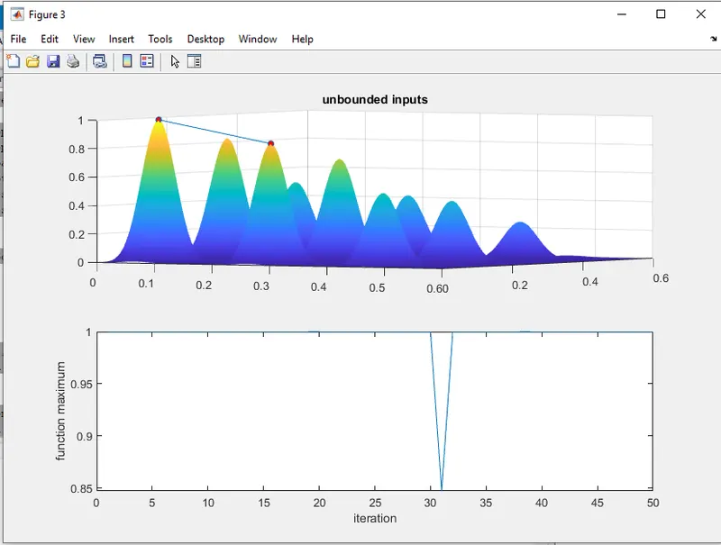
As we observe we finnd the exact optimum Maxima values in this study