Week 7 - Simulation of a 1D Super-sonic nozzle flow simulation using Macormack Method
Simulation of a 1D Super-sonic nozzle flow simulation using Maccormack Method
Before solving the problem, lets understand what is it we are solving for and how?
We are to solve for a steady state 1D supersonic nozzle flow and simulate the results for the same.
The nozzle in consideration is a 'convergent-divergent nozzle' or simply 'C-D nozzle'. In a C-D nozzle, if the flow entering is subsonic, the flow at throat is sonic or supersonic and it continues to be supersonic in the divergent section. If the flow entering the convergent section is supersonic, the inverse happpens in ddivergent section i.e.: flow will be subsonic in divergent section.
The flow in our consideration is a steady isentropic flow through C-D nozzle with subsonic flow in convergent section, sonic at the throat and supersonic in the divergent section. The properties are defined as follows:
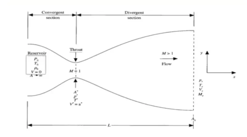
| Property | Inlet | Outlet |
| Pressure | `P_o` | `P_e` |
| Temperature | `T_o` | `T_e` |
| Area | `Ararroo` | `A_e` |
| Velocity | `V~~0` | `V_e` |
| Density | `rho_o` | `rho_e` |
We assume the properties at a given distance in the nozzle are uniform across the cross section. So, although the area of nozzle is a function of distance along the flow direction and flow is 2D in reality, we have assumed the flow to be varying along the flow direction only i.e 1D. Such a flow is called as Quasi-one-dimensional flow.
The Governing Equations for the Quasi-one -dimensional flow are as follows:
1)Continuity: `rho_1A_1V_1=rho_2A_2V_2`
2)Momentum: `p_1A_1+rho_1A_1V_1^2+int_(A_1)^(A_2)pdA=p_2A_2+rho_2A_2V_2^2`
3)Energy: `h_1+(V_1^2)/2=h_2+(V_2^2)/2`
apart from these, we have,
4)Equation of state: `p=rhoRT`
5)perfect gas relation: `h=c_PT`
CONSERVATIVE FORM:
Considering a fixed control volume and applying the physical principals, the resulting equation we get is flow equations in conservative and integral form.
1)Continuity equation: `del/(delt)intintintrhodccV+intintrhoV.dS=0`
`del/(delt)intintintrhodccV=del/(delt)(rhoAdx)` for `dxrarr0`
similarly,
`intintrhoV.dS=-rhoVA+(rho+drho)(A+dA)(V+dV)`
`=rhoAdV+rhoVdA+AVdrho = d(rhoAV)` for `dxrarr0`.
which gives `del/(delt)(rhoAdx)+d(rhoAV)=0`
Dividing by dx, the 2nd term on the LHS becomes a partial derivative as `dxrarr0`.
`del/(delt)(rhoA)+del/(delx)(rhoAV)=0` is the partial differential continuity equation for quasi-one-dimensional flow in conservative form.
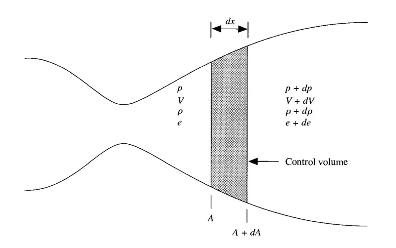
2)Momentum Equation: `del/(delt)intintint(rhou)dccV+intint(rhouV).dS=-intint(p.dS)_x`
`del/(delt)intintintrhoudccV=del/(delt)(rhoVAdx)` for `dxrarr0`
`intintrhouV.dS=-rhoV^2A+(rho+drho)(A+dA)(V+dV)^2`
`intint(p.dS)_x=-pA+(p+dp)(A+dA)-2p((dA)/2)`the last term on RHS is due to pressure from top and bottom faces of the control volume. Substituting all the terms back in the integral momentum equation gives:
`del/(delt)(rhoAVdx)+d(rhoV^2A)=-Adp`
Dividing by dx, the 2nd term on the LHS and RHS term become partial derivatives as `dxrarr0`.
`del/(delt)(rhoAV)+(del(rhoV^2A))/(delx)=-A(delp)/(delx)` is the partial differential momentum equation for quasi-one-dimensional-flow in coservative form.
3)Energy Equation: `del/(delt)intintintrho(e+V^2/2)dccV+intintrho(e+V^2/2)V.dS=-intint(pV).dS_x`
`del/(delt)intintintrho(e+V^2/2)dccV`= `del/(delt)[rho(e+V^2/2)Adx]` for `dxrarr0`
`intintrho(e+V^2/2)V.dS`=`-rho(e+V^2/2)VA+(rho+drho)(e+de+(V+dV)^2/2)(V+dV)(A+dA)`
`intint(pV).dS_x`=`-pVA+(p+dp)(V+dV)(A+dA)-2(pV(dA)/2)`
Substituting all the terms back in the integral momentum equation gives:
`del/(delt)[rho(e+V^2/2)Adx]+d[rho(e+V^2/2)VA]=-d(pAV)`
Dividing by dx, the 2nd term on the LHS and RHS term become partial derivatives as `dxrarr0`.
`del([rho(e+V^2/2)Adx])/(delt)+(del[rho(e+V^2/2)VA])/(delx)=-(del(pAV))/(delx)` is the partial differential energy equation for quasi-one-dimensional-flow in conservative flow.
NON-CONSERVATIVE FORM:
1)Continuity Equation: Considering the conservative form derived above `del/(delt)(rhoA)+del/(delx)(rhoAV)=0`. Opening up the brackets and seperating each term using chain rule, we get:
`A(delrho)/(delt)+rhocancel((delA)/(delt))+AV(delrho)/(delx)+Arho(delV)/(delx)+rhoV(delA)/(delx)=0`
Since A is a function of x only.
Dividing by A on both sides,
`(delrho)/(delt)+(rhoV)/A(delA)/(delx)+rho(delV)/(delx)+V(delrho)/(delx)=0`
simplifying further,
`(delrho)/(delt)+rhoV(del(lnA))/(delx)+(del(rhoV))/(delx)=0` is the partial differential continuity equation of quasi-one-dimensional-flow in non-conservative form.
2)Momentum Equation: By manipulating the conservative Momentum equation we can obtain the non-conservative form.
Multiplying the conservative continuity equation by 'V' on both sides and substracting it from the conservative momentum equation,
`del/(delt)(rhoAV)-V(del(rhoA))/(delt)-V(del(rhoAV))/(delx)+(del(rhoV^2A))/(delx)=-A(delp)/(delx)`
Expanding and cancelling like terms,
`rho(delV)/(delt)+rhoV(delV)/(delx)=-(delp)/(delx)` is the partial differential momentum equation of quasi-one-dimensional-flow in non-conservative form.
3)Energy Equation: By manipulating the conservative Energy equation we can obtain the non-conservative form.
Multiplying the conservative Momentum equation by 'V' on both sides and substracting it from the conservative energy equation,
`del([rho(e+V^2/2)Adx])/(delt)+(del[rho(e+V^2/2)VA])/(delx)-(del[rhoV^2/2A])/(delt)-(del[rhoV^3/2A])/(delx)=-(del(pAV))/(delx)+AV(delp)/(delx)`
`(del(rhoeA))/(delt)+(del(rhoVeA))/(delx)=-p(del(AV))/(delx)` which is the partial differential energy equation of quasi-one-dimensional-flow in non-conservative form.
These equations are used in discretized form (conservative/non conservative) for a large number of time-steps to give a steady state solution of the flow field. While there are other methods we can use to solve for the flow field, we are going to use the MACCORMACK Technique to solve the problem using both conservative and non-conservative forms of the governing equations.
MACCORMACK'S TECHNIQUE: First introduced in 1969, it became the most popular explicit finite difference technique for solving fluid flow problems for the next 15 years. Though being replaced by more accurate and sophisticated solvers, it gives fairly satisfactory results for some less complicated flows like, supersonic fluid flow in a Convergent-Divergent nozzle.
The advantage of MACCORMACK'S technique over other time-marching techniques is that it doesn't require us to calculate the second derivative term to achieve second order accuracy.
This is achieved as :
`rho_(i,j)^(t+Deltat)=rho_(i,j)^t+((delrho)/(delt))_(av)Deltat`
here, 2nd order accuracy is captured by the `((delrho)/(delt))_(av)` term. It is defined as the average of the differential calculated using forward-difference and backward-difference schemes. i.e:
`1/2{((delrho)/(delt))_(i,j)^t+(bar(delrho)/(delt))_(i,j)^(t+Deltat)}`
where, `((delrho)/(delt))_(i,j)^t` represents the finite forward-difference term while `(bar(delrho)/(delt))_(i,j)^(t+Deltat)` represents the finite bacward-difference term.
Procedure:
Firstly, based on the initial conditions the forward-difference derivatives are calculated using the governing equations. This is then followed by a predictor step where predicted vlaues of the flow variable is calculated using the forward-difference derivative and initial conditions,
`barrho_(i,j)^((t+Deltat))=rho_(i,j)^t+((delrho)/(delt))_i^tDeltat`
Once predicted values are calculated, the backward-difference derivative is calculated using the governing equations and the predictor step values. This is called the corrector step.
It is then followed by calculating the average-derivative term as `1/2{((delrho)/(delt))_(i,j)^t+(bar(delrho)/(delt))_(i,j)^(t+Deltat)}`.
Finally, the values for next time are updated using the previous time step values and the average-derivative term,
`rho_(i,j)^(t+Deltat)=rho_(i,j)^t+((delrho)/(delt))_(av)Deltat`
This whole procedure is carried for all flow variables like velocity, temperature, etc. for a definite and sufficiently large time period to give steady state results.
One important thing to note is that in case of conservative form of governing equation it is not the primitive variables (density, velocity, temperature) that we solve for. Rather, it is the derived variables, which is a combination of more than one primitive variable, is obtained as the solution. From these derived varibales we calculate our primitives. For eg.: instead of density '`rho`' we have `U_1=rhoA`, `U_2=rhoAV`, `U_3=rho(e/(gamma-1)+gamma/2V^2)A` are obtained as solution. `rho=U_2/U_1` is how we obtain values of primitives.
The Code:
Two seperate programs have been written, one for conservative and another for non-conservative approach, to avoid mixup of variables.
Non-Conservative:
Lines 5-18: We start by defining the inputs,
%%
%Inputs
n=31;
x=linspace(0,3,n);
cp=1;                                              %specific heat at constan pressure in kJ/kg-K.
dx=x(2)-x(1);                                      %node spacing
cv=0.718;                                          %specific heat at constan volume in kJ/kg-K.
gamma=cp/cv;                                       %ratio of specific heats.
A=1+2.2*(x-1.5).^2;                                %Area variation along the length of the nozzle.

[T_initial_nc]=1-(0.2314*x);                       %Initial condition of temperature at t=0 as a function of x (dimensionless).
[rho_initial_nc]=1-(0.314*x);                      %Initial condition of density at t=0 as a function of x (dimensionless).
[V_initial_nc]=(0.1+1.09.*x).*(T_initial_nc).^0.5; %Initial condition of velocity at t=0 as a function  of x (dimensionless).
Line 30: The outermost 'for' loop is the time loop running the code below for given number time steps (in our case 1000).
% Variation of variable-distribution with time.
f1=figure('Name',' Normalized Variables VS Length (Non-Conservative)');
t=0;
for l=1:1000
    V_old=V_nc;
    T_old=T_nc;
    rho_old=rho_nc;

    dt_nc=min((C.*dx)./((T_nc.^0.5)+V_nc));
    dt(l)=dt_nc;                                      % will be useful for figure3 'for' loop
    t=t+dt(l);
    %Forward Difference
    for i=2:n-1
        V1=V_nc(i);
        V2=V_nc(i+1);
        T1=T_nc(i);
        T2=T_nc(i+1);
        rho1=rho_nc(i);
        rho2=rho_nc(i+1);
        A1=A(i);
        A2=A(i+1);
        [dV_dt_p,dT_dt_p,drho_dt_p]=fwd_diff_der(V1,V2,T1,T2,rho1,rho2,A1,A2,dx,gamma);%function callout to get forward-difference derivative terms.
        fdV_dt(i)=dV_dt_p;                         %storing forward-difference derivative of velocity.
        fdT_dt(i)=dT_dt_p;                         %storing forward-difference derivative of temperature.
        fdrho_dt(i)=drho_dt_p;                     %storing forward-difference derivative of density.
        V_nc(i)=V_nc(i)+((fdV_dt(i))*dt_nc);       %Predicted values of velocity.
        T_nc(i)=T_nc(i)+((fdT_dt(i))*dt_nc);       %Predicted values of tmperature.
        rho_nc(i)=rho_nc(i)+((fdrho_dt(i))*dt_nc); %Predicted values of density.
    end

    %CORRECTOR STEP

    %backward difference spatial derivatives.

    for i=2:n-1
        V3=V_nc(i-1);
        V4=V_nc(i);
        T3=T_nc(i-1);
        T4=T_nc(i);
        rho3=rho_nc(i-1);
        rho4=rho_nc(i);
        A3=A(i-1);
        A4=A(i);
        [dV_dt_c,dT_dt_c,drho_dt_c]=bwd_diff_der(V3,V4,T3,T4,rho3,rho4,A3,A4,dx,gamma); %function callout to get backward-difference derivative terms.
        bdV_dt(i)=dV_dt_c;                         %storing backward-difference derivative of velocity.
        bdT_dt(i)=dT_dt_c;                         %storing backward-difference derivative of temperature.
        bdrho_dt(i)=drho_dt_c;                     %storing backward-difference derivative of density.
    end

    % average gradient values
    for i=2:n-1
        avg_dV_dt(i)=0.5*(fdV_dt(i)+bdV_dt(i));    %average derivative of velocity.
        avg_dT_dt(i)=0.5*(fdT_dt(i)+bdT_dt(i));    %average derivative of temperature.
        avg_drho_dt(i)=0.5*(fdrho_dt(i)+bdrho_dt(i));%average derivative of density.
    end

    %corrected values of variables
    for i=2:n-1
        V_nc(i)=V_old(i)+(avg_dV_dt(i).*dt_nc);     %obtaining velocity values for the next time step.
        T_nc(i)=T_old(i)+(avg_dT_dt(i).*dt_nc);     %obtaining temperature values for the next time step.
        rho_nc(i)=rho_old(i)+(avg_drho_dt(i).*dt_nc);%obtaining density values for the next time step.
        if i==16
            V16(l)=V_nc(i);                           % normalized velocity at the throat.
            T16(l)=T_nc(i);                           % normalized temperature at the throat.
            rho16(l)=rho_nc(i);                       % normalized density at the throat.
        end
    end

    V_nc(1)=(2*V_nc(2))-V_nc(3);                      % extrapolating  inlet velocity.
    V_nc(31)=(2*V_nc(30))-V_nc(29);                   % extrapolating outlet velocity

    T_nc(31)=(2*T_nc(30))-T_nc(29);                   % extrapolating inlet temperature.
    rho_nc(31)=(2*rho_nc(30))-rho_nc(29);             % extrapolating inlet density.

    P=rho_nc.*T_nc;                                   % Normalized Pressure distribution.
    M=V_nc./(T_nc.^0.5);                              % Mach Number distribution.

    for i=1:n
        mass(i)=rho_nc(i)*A(i)*V_nc(i);               % mass distribution across the nozzle.
    end

    P16=rho16.*T16;                                   % Normalized Pressure at the throat.

    str=sprintf('Time = %.2f seconds',t);

    %plotting the flow field variables for each time step.
    subplot(3,2,1)
    plot(x,V_nc)
    ylim([0 2])
    grid on
    xlabel('x')
    ylabel('V/a_o')
    pause(0.0005)

    subplot(3,2,2)
    plot(x,T_nc)
    ylim([0 2])
    grid on
    xlabel('x')
    ylabel('T/T_o')
    pause(0.0005)

    subplot(3,2,3)
    plot(x,rho_nc)
    ylim([0 2])
    grid on
    xlabel('x')
    ylabel('rho/rho_o')
    pause(0.0005)

    subplot(3,2,4)
    plot(x,P)
    ylim([0 2])
    grid on
    xlabel('x')
    ylabel('P/P_o')
    pause(0.0005)

    subplot(3,2,5)
    plot(x,M)
    xlim([0 3])
    grid on
    xlabel('x')
    ylabel('Mach Number (M)')
    pause(0.0005)

    subplot(3,2,6)
    plot(x,mass)
    ylim([0 2])
    grid on
    xlabel('x')
    ylabel('Mass Flow Rate')
    pause(0.0005)

    sgtitle(str);

    cntr(l)=getframe(f1);
end
The code inside the for loop contains the code for calculating the forward-difference derivative, backward-difference derivative, average-derivative and susiquently the next time step values for the variables. At the end plotting the resulting flow field for all time steps.
The following function callouts for calculating forward and backward difference derivatives were used:
%%function to calculate forward-difference derivatives
function [dV_dt_p, dT_dt_p, drho_dt_p]=fwd_diff_der(V1,V2,T1,T2,rho1,rho2,A1,A2,dx,gamma)

term1=(V2-V1)/(dx);
term2=(log(A2)-log(A1))/(dx);
term3=(rho2-rho1)/(dx);
term4=(T2-T1)/(dx);

term5=(term1)+(V1)*(term2);

dV_dt_p=-(V1)*(term1)-(1/gamma)*((term4)+(T1/rho1)*(term3));
dT_dt_p=-(V1)*(term4)-(gamma-1)*(T1)*(term5);
drho_dt_p=-(rho1)*(term1)-(rho1)*(V1)*(term2)-V1*(term3);
end
%%function to calculate backward-difference derivatives
function [dV_dt_c, dT_dt_c, drho_dt_c]=bwd_diff_der(V3,V4,T3,T4,rho3,rho4,A3,A4,dx,gamma)

term1=(V4-V3)/(dx);
term2=(log(A4)-log(A3))/(dx);
term3=(rho4-rho3)/(dx);
term4=(T4-T3)/(dx);
term5=(term1)+(V4)*(term2);

dV_dt_c=-(V4)*(term1)-(1/gamma)*((term4)+(T4/rho4)*(term3));
dT_dt_c=-(V4)*(term4)-(gamma-1)*(T4)*(term5);
drho_dt_c=-(rho4)*(term1)-(rho4)*(V4)*(term2)-V4*(term3);
end
Line 166-172: Code for saving the animation obtained from above code sections.
%saving the animation for the above plot (figure 1).
f2=figure('Name',' Normalized Primitives VS Length (Non-Conservative)');
movie(cntr);
animation=VideoWriter('Normalized Primitives VS Normalized Length (31 gridpoints).avi');
open(animation);
writeVideo(animation,cntr);
close(animation);
Line 174-222: Plotting for the variation in variables at the throat section of the C-D nozzle.
% Variation of Variables ath the throat section with time.
f3=figure('Name','Variation of Normalized Properties at Throat (Non-Conservative)');
t=0;
for l=1:1000
    t=t+dt(l);
    str=sprintf('Time = %.2f seconds',t);

    subplot(4,1,1)
    plot(l,V16(l),'Color','b','Marker','o','MarkerSize',0.4)
    ylim([0 2])
    xlim([0 1000])
    grid on
    xlabel('Number of time steps')
    ylabel('(V/a_o)_t_h_r_o_a_t')
    hold on
    pause(0.00001)

    subplot(4,1,2)
    plot(l,T16(l),'Color','b','Marker','o','MarkerSize',0.4)
    ylim([0 2])
    xlim([0 1000])
    grid on
    xlabel('Number of time steps')
    ylabel('(T/T_o)_t_h_r_o_a_t')
    hold on
    pause(0.00001)

    subplot(4,1,3)
    plot(l,rho16(l),'Color','b','Marker','o','MarkerSize',0.4)
    ylim([0 2])
    xlim([0 1000])
    grid on
    xlabel('Number of time steps')
    ylabel('(rho/rho_o)_t_h_r_o_a_t')
    hold on
    pause(0.00001)

    subplot(4,1,4)
    plot(l,P16(l),'Color','b','Marker','o','MarkerSize',0.4)
    ylim([0 2])
    xlim([0 1000])
    grid on
    xlabel('Number of time steps')
    ylabel('(P/P_o)_t_h_r_o_a_t')
    hold on
    pause(0.00001)

    sgtitle(str);
end
Conservative:
Line 5-17 : Defining inputs,
%%Inputs
n=31;                                              %number of node points.
x=linspace(0,3,n);
cp=1;                                              %specific heat at constan pressure in kJ/kg-K.
dx=x(2)-x(1);                                      %node spacing
cv=0.718;                                          %specific heat at constan volume in kJ/kg-K.
gamma=cp/cv;                                       %ratio of specific heats.
A=1+2.2*(x-1.5).^2;                                %Area variation along the length of the nozzle.

for i=1:n                                          %Defining initial conditions.
    if le(x(i),0.5) && ge(x(i),0)
        rho_initial_c(i)=1;
        T_initial_c(i)=1;
    end
    if gt(x(i),0.5) && le(x(i),1.5)
        rho_initial_c(i)=1-0.366*(x(i)-0.5);
        T_initial_c(i)=1-0.167*(x(i)-0.5);
    end
    if gt(x(i),1.5) && le(x(i),3)
       rho_initial_c(i)=0.634-0.3879*(x(i)-1.5);
       T_initial_c(i)=0.833-0.3507*(x(i)-1.5);
    end
    V_initial_c(i)=0.59/(rho_initial_c(i)*A(i));
end

rho_c=rho_initial_c;
T_c=T_initial_c;
V_c=V_initial_c;
C=0.5;

U1=rho_c.*A;                                        %solution variables U1, U2 and U3.
U2=rho_c.*A.*V_c;
U3=rho_c.*((T_c./(gamma-1))+((gamma/2).*V_c.^2)).*A;
Line 44-201: The outermost 'for' loop is the time loop running the code below for given number time steps (in our case 1000).
for l=1:1000
    dt_c=min((C.*dx)./((T_c.^0.5)+V_c));            %time step calculation.
    dt(l)=dt_c;                                     %will be useful for figure6 for loop.
    t=t+dt(l);
    U1_old=U1;                                      %values of U1, U2, U3 at previous time step.
    U2_old=U2;
    U3_old=U3;

    for i=1:n                                       %calculating variables at internal grid points.
        u1=U1(i);
        u2=U2(i);
        u3=U3(i);
        [f1,f2,f3]=flux_conservative(u1,u2,u3,gamma);
        F1(i)=f1;                                   %Flux terms F1, F2 and F3.
        F2(i)=f2;
        F3(i)=f3;
    end

    %For loop for calculating forward difference derivative of solution variables and updated solution variables
    for i=2:n-1
        J2=(1/gamma)*(rho_c(i))*(T_c(i))*(A(i+1) - A(i))/dx;
        g1=F1(i);
        g2=F1(i+1);
        h1=F2(i);
        h2=F2(i+1);
        k1=F3(i);
        k2=F3(i+1);
        dU1_dt_pr(i)=-(g2-g1)/dx;
        dU2_dt_pr(i)=-((h2-h1)/dx)+J2;
        dU3_dt_pr(i)=-(k2-k1)/dx;
        U1(i)=U1(i)+((dU1_dt_pr(i))*dt_c);
        U2(i)=U2(i)+((dU2_dt_pr(i))*dt_c);
        U3(i)=U3(i)+((dU3_dt_pr(i))*dt_c);
        rho_c(i)=U1(i)/A(i);
        T_c(i)=(gamma-1)*((U3(i)/U1(i))-((gamma/2)*(U2(i)/U1(i))^2));
    end

    %For loop for calculating updated flux terms.
    for i=1:n
        u1=U1(i);
        u2=U2(i);
        u3=U3(i);
        [f1,f2,f3]=flux_conservative(u1,u2,u3,gamma);
        F1(i)=f1;
        F2(i)=f2;
        F3(i)=f3;
    end

    %For loop for calculating backward difference derivaative of solution
    %variables.
    for i=2:n-1
        J2=(1/gamma)*(rho_c(i))*(T_c(i))*(A(i) - A(i-1))/dx;
        g3=F1(i-1);
        g4=F1(i);
        h3=F2(i-1);
        h4=F2(i);
        k3=F3(i-1);
        k4=F3(i);
        dU1_dt_cr(i)=-(g4-g3)/dx;
        dU2_dt_cr(i)=-((h4-h3)/dx)+J2;
        dU3_dt_cr(i)=-(k4-k3)/dx;
    end

    %For loop for calculating average differential terms ussing forward and
    %backward differential terms.
     for i=2:n-1
        avg_dU1_dt(i)=0.5*(dU1_dt_pr(i)+dU1_dt_cr(i));
        avg_dU2_dt(i)=0.5*(dU2_dt_pr(i)+dU2_dt_cr(i));
        avg_dU3_dt(i)=0.5*(dU3_dt_pr(i)+dU3_dt_cr(i));
     end

     %calculating values of variables at current time step.
     for i=2:n-1
        U1(i)=U1_old(i)+(avg_dU1_dt(i).*dt_c);
        U2(i)=U2_old(i)+(avg_dU2_dt(i).*dt_c);
        U3(i)=U3_old(i)+(avg_dU3_dt(i).*dt_c);
        rho_c(i)=U1(i)/A(i);
        V_c(i)=U2(i)/U1(i);
        T_c(i)=(gamma-1)*((U3(i)/U1(i))-((gamma/2)*(V_c(i))^2));
        if i==16                                     %loop for saving values of primitives at throat section for every time step.
           rho_c_16(l)=rho_c(i);                     %normalized Density at the throat area.
           V_c_16(l)=V_c(i);                         %normalized Velocity at the throat area.
           T_c_16(l)=T_c(i);                         %normalized Temperature at the throat area.
        end
     end

     U2(1)=2*U2(2)-U2(3);                            %since U2 and U3 are floating variables value are extrapolated at 1st grid point.
     U3(1)=rho_c(1)*((T_c(1)/(gamma-1))+((gamma/2)*V_c(1)^2))*A(1);

     U2(31)=2*U2(30)-U2(29);                         %extrapolating values of variables at the boundaries.
     U1(31)=2*U1(30)-U1(29);
     U3(31)=2*U3(30)-U3(29);

     rho_c=U1./A;                                    %value of primitive variable -normalized density- at steady state.
     V_c=U2./U1;                                     %value of primitive variable -normalized velocity- at steady state.
     T_c=(gamma-1)*((U3./U1)-((gamma/2)*(V_c).^2));  %value of primitive variable -normalized temperature- at steady state.
     P_c=rho_c.*T_c;                                 % Normalized Pressure distribution.
     M_c=V_c./(T_c.^0.5);                            % Mach Number distribution.
     for i=1:n
        mass_c(i)=rho_c(i)*A(i)*V_c(i);              % mass distribution across the nozzle.
     end
     P_c_16=rho_c_16.*T_c_16;                        % Normalized Pressure at the throat.

     str=sprintf('Time = %.2f seconds',t);

     %Ploting the results
     subplot(3,2,1)
     plot(x,V_c)
     ylim([0 2])
     grid on
     xlabel('x')
     ylabel('V/a_o')
     pause(0.0005)

     subplot(3,2,2)
     plot(x,T_c)
     ylim([0 2])
     grid on
     xlabel('x')
     ylabel('T/T_o')
     pause(0.0005)

     subplot(3,2,3)
     plot(x,rho_c)
     ylim([0 2])
     grid on
     xlabel('x')
     ylabel('rho/rho_o')
     pause(0.0005)

     subplot(3,2,4)
     plot(x,P_c)
     ylim([0 2])
     grid on
     xlabel('x')
     ylabel('P/P_o')
     pause(0.0005)

     subplot(3,2,5)
     plot(x,M_c)
     xlim([0 3])
     grid on
     xlabel('x')
     ylabel('Mach Number (M)')
     pause(0.0005)

     subplot(3,2,6)
     plot(x,mass_c)
     ylim([0 2])
     grid on
     xlabel('x')
     ylabel('Mass Flow Rate')
     pause(0.0005)

     sgtitle(str);

     cntr(l)=getframe(f4);
end
The code inside the for loop contains the code for calculating the forward-difference derivative, backward-difference derivative, average-derivative and susiquently the next time step values for the variables. At the end plotting the resulting flow field for all time steps.
The following function callout for calculating the flux terms was used:
function [f1,f2,f3]=flux_conservative(u1,u2,u3,gamma)
term1=(u2^2)/u1;
term2=(gamma-1)/gamma;
term3=(gamma/2)*term1;
term4=(gamma*u2*u3)/u1;
term5=gamma*(gamma-1)/2;
term6=(u2^3)/u1^2;

f1=u2;
f2=term1+term2*(u3-term3);
f3=term4-(term5*term6);
end
Line 203-208: Code for saving the animation obtained from above code sections.
f5=figure('Name',' Normalized Primitives VS Length (Conervative)');
movie(cntr);
animation=VideoWriter('Normalized Primitives VS Normalized Length (conservative) (31grid points).avi');
open(animation);
writeVideo(animation,cntr);
close(animation);
Line 210-257: Plotting for the variation in variables at the throat section of the C-D nozzle.
f6=figure('Name','Variation of Normalized Properties at Throat (Consevative)');
t=0;
for l=1:1000
    t=t+dt(l);
    str=sprintf('Time = %.2f seconds',t);

    subplot(4,1,1)
    plot(l,V_c_16(l),'Color','b','Marker','o','MarkerSize',0.4)
    ylim([0 2])
    xlim([0 1000])
    grid on
    xlabel('Number of time steps')
    ylabel('(V/a_o)_t_h_r_o_a_t')
    hold on
    pause(0.00005)

    subplot(4,1,2)
    plot(l,T_c_16(l),'Color','b','Marker','o','MarkerSize',0.4)
    ylim([0 2])
    xlim([0 1000])
    grid on
    xlabel('Number of time steps')
    ylabel('(T/T_o)_t_h_r_o_a_t')
    hold on
    pause(0.00005)

    subplot(4,1,3)
    plot(l,rho_c_16(l),'Color','b','Marker','o','MarkerSize',0.4)
    ylim([0 2])
    xlim([0 1000])
    grid on
    xlabel('Number of time steps')
    ylabel('(rho/rho_o)_t_h_r_o_a_t')
    hold on
    pause(0.00005)

    subplot(4,1,4)
    plot(l,P_c_16(l),'Color','b','Marker','o','MarkerSize',0.4)
    ylim([0 2])
    xlim([0 1000])
    grid on
    xlabel('Number of time steps')
    ylabel('(P/P_o)_t_h_r_o_a_t')
    hold on
    pause(0.00005)

    sgtitle(str);
end
RESULTS:
Non-Conservative:
Following plots were obtained
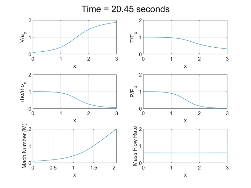
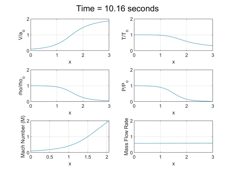
Left figure is for 31 grid points and Right figure is for 61 grid points.
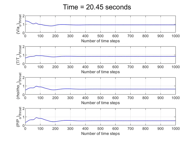
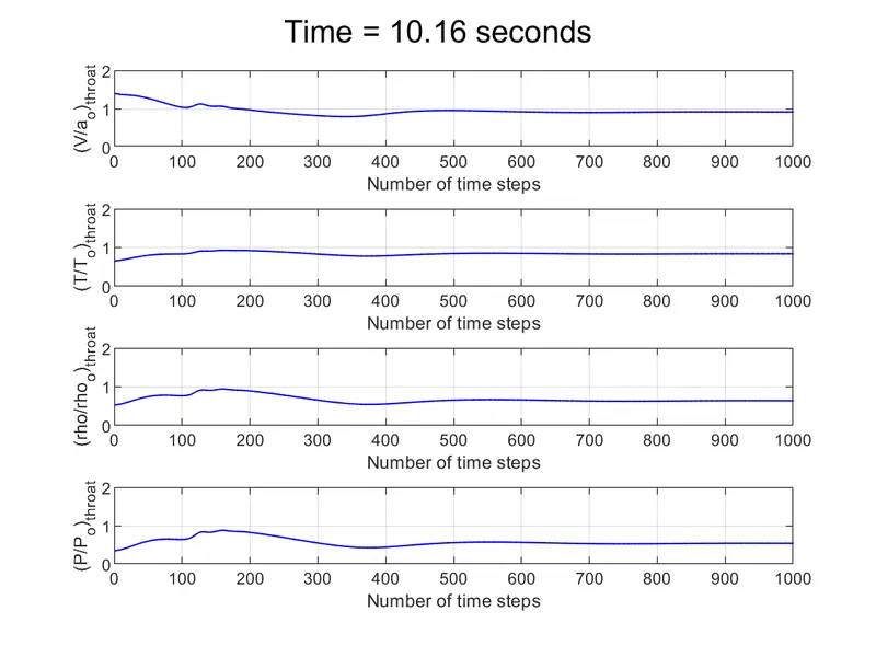
Left figure is for 31 grid points and Right figure is for 61 grid points.
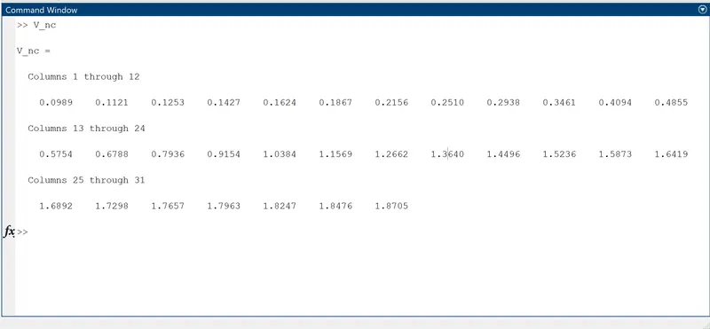
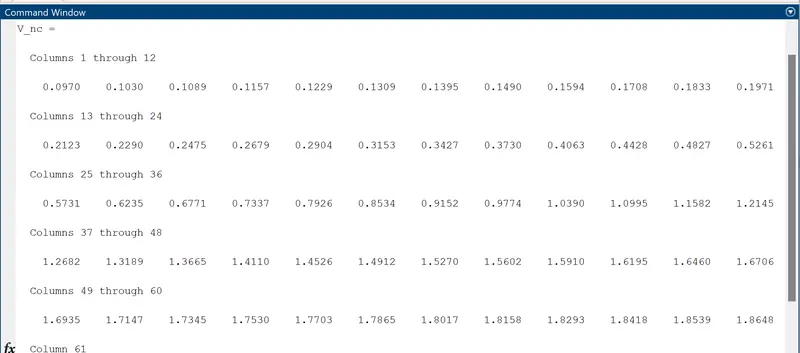
Left figure is for 31 grid points and Right figure is for 61 grid points.
Conservative:
Following plots were obtained
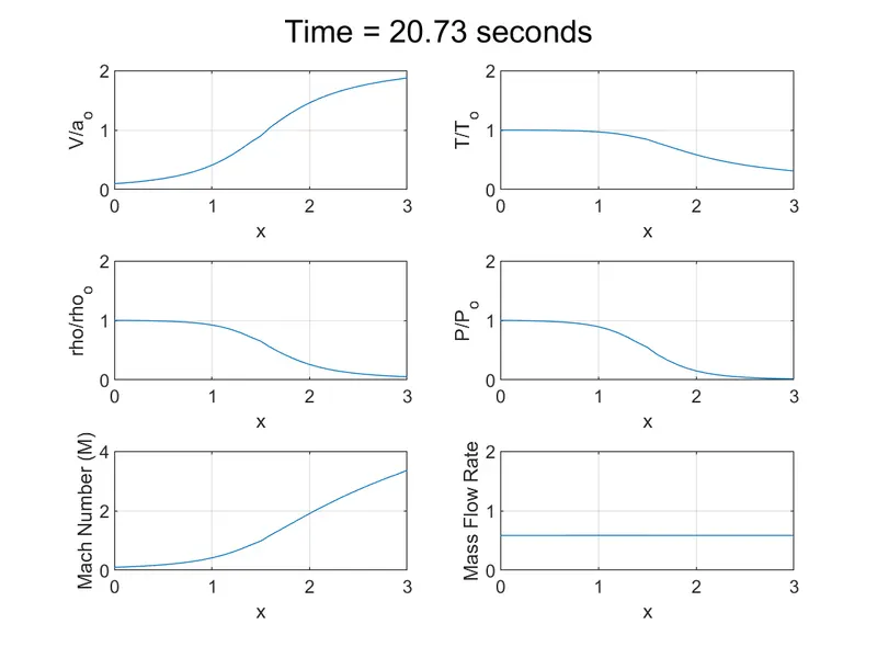
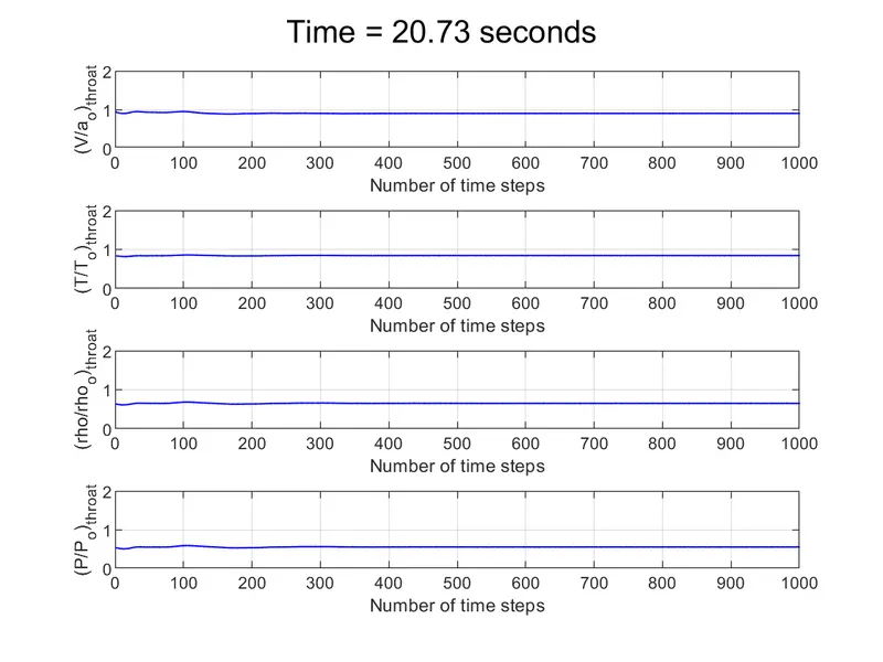
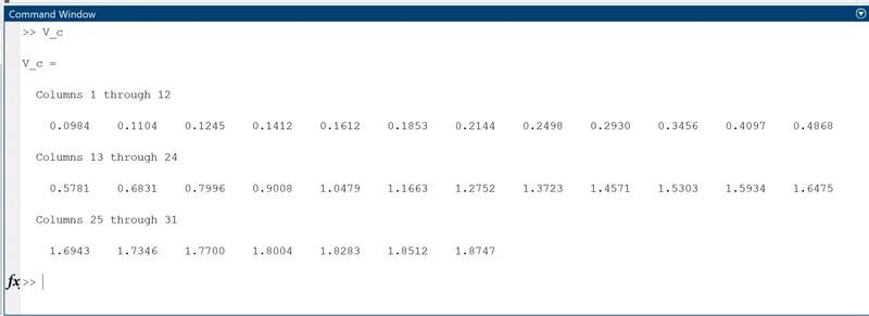
OBSERVATIONS AND CONCLUSION:
Considering values of variables at some specific points to make a comaprison between different plots obtained by varying certain parameters, following observations and conclusions can be made:
- On first glance on the steady state field variables plot, it is consistent with the theory of C-D nozzle. Since the flow is subsonic at the convergent region sonic at the throat the flow must be supersonic in the divergent section. i.e. Velocity and Mach Number increases along the flow direction, Pressure and Temperature decreases along the flow direction.
- Going by the plots of conservative and non-conservative governing equation, we see the plots are identical. It must be so as they were based on same physical principle also they are same equation theoretically. Its just that each of them are required to be solved in a particular manner due to mathematical differences.
For eg. considering velocity at the inlet i.e. (V_nc)inlet and (V_c)inlet, the difference is of 0.0005.
Similarly at the outlet the difference is of 0.0042 & at throat a difference of 0.0146 respectively. - Looking on variation of flow variables at throat for all the time steps it is observed that the conservative governing equation converges faster than non-conservative governing equation.
- We also tried to solve the non-conservative equations using different number of grid points- 31 and 61 grid points. The results were marginally improved compared to the amount of computational effort it required. The computational time for same number of time steps but almost double the grid points was also doubled (from 10 seconds to 20 seconds).
This suggests that the solution has achieved grid independence at 31 grid points with satisfactory level of accuracy.
References:
- Computational Fluid Dynamics the Basics with Applications by John David Anderson (Chapter 2, 6 & 7) .