Week 7 - Simulation of a 1D Super-sonic nozzle flow simulation using Macormack Method

# Simulation of a 1D Super-sonic nozzle flow simulation using Macormack Method #

As we know the considering Steady Isentropic flow through a convergent-divergent nozzle.

• Steady:- The velocity remais constant at a particular point it does not change with time.
• Isentropic Flow:- When the gas is forced through a tube, the gaseous molecules are dflected by the tubes wall. If the speed of gas is much less than the speed of Sound the gas density remains constant & velocity flow increase. As we speed of flow similar to speed of sound, compresibility effect on the gas are to be consider. The density of gas becomes position dependent. While considering flow through tube, if the flow is very gradually compressed (i.e. area decrease) & gradually expands (i.e. area increase) the flow condition are restored (i. e. return to the initial posiition). So the process is reversible process. According to the 2nd law of thermodynamic there is a reversible & adiabatic flow, constant value of entropy is maintained this is ISENTROPIC flow.

As we know the considering Steady Isentropic flow through a convergent-divergent nozzle. The flow at inlet to nozzle comes from reservoir pressure & temperature are denoted by (`P_0 & T_0`) respectively. The C/A of reservoir at inlet is large (`Ararrinfty`) and hence the velocity is small (`Vrarr0`).

The flow expands isentropically to supersonic speed at the nozzle exit, where the exit pressure, temp, velocity & mach numb. are denoted by (`P_e, T_e, V_e, M_e`) resp.

The flow is locally subsonic in the convergent section of nozzle, sonic at throat (minimum area), & supersonic at divergent section. The sonic flow (M=1) at the throat means local velocity at this location is equal to local speed of sound i.e.(`V=V^ast=a^ast`). Similarly, the sonic flow values of pressure and remprature are denoted by (`P^ast & T^ast`) resp.

The area of sonic throat is denoted by `A^ast`

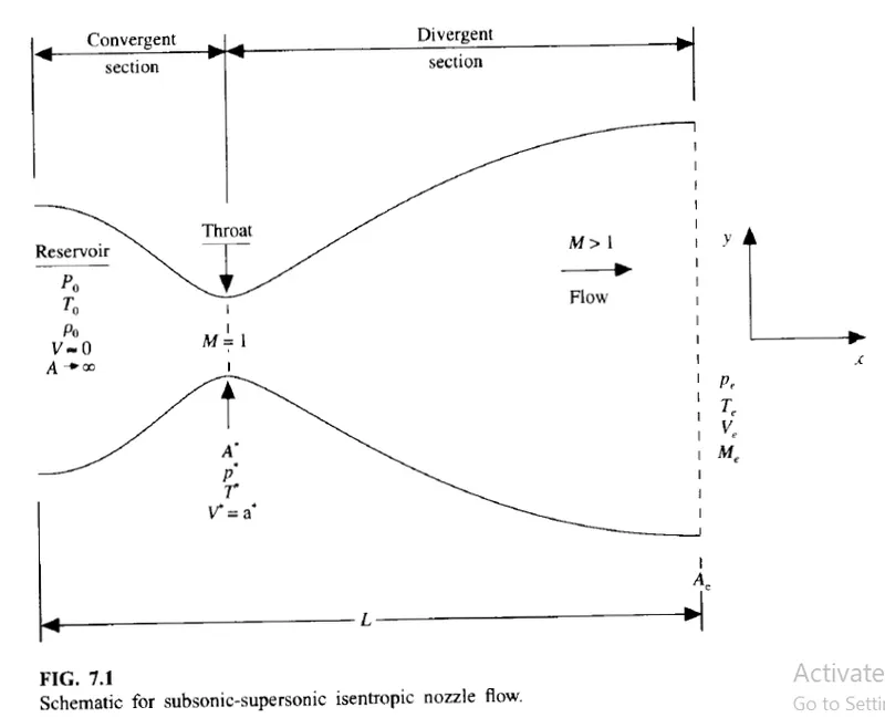
We assume that at a given section, where the C/A area is A, the flow properties are uniform of distance along the nozzle, x, and the reality flow field is 2D (flow varies in 2D xy space), we make the assumption that the flow properties vary only with x; this is the tantamount to assuming uniform flow properties across any given cross section such flow is defined as quasi-one-dimensional flow.

INLET:

1. `P_0`= Stagnation Pressure
2. `T_0`= Stagnation Temp
3. `rho_0`= Stagnation density
4. `Vrarr0` Velocity equals to 0
5. `Ararrinfty`Area at reservoir is large
6. `M_0 = (Mlt1)` Mach no. of subsonic flow at reservoir

THROAT:

1. `A^ast`= Area of sonic throat
2. `P^ast`=Press of sonic flow at throat
3. `T^ast`= Temp of sonic flow at throat
4. `V^ast`=Vel of sonic flow at throat
5. `a^ast`=sound vel. of sonic flow at throat
6. `M^ast`= Mach no. of sonic flow at throat (M=1)

OUTLET:

1. `P_e`=Press of supersonic speed at outlet,
2. `T_e`=Temp of supersonic speed at outlet
3. `V_e`=Vel.of supersonic speed at outlet
4. `A_e`= Area of supersonic speed at outlet
5. `rho_e`=Density of supersonic speed at outlet
6. `M_e`=Mach no. of supersonic speed at outlet

The governing, continuity, momentum & energy equation for this quasi-one dimensional flow, steady isentropic

1. `rho_1,V_1,A_1=rho_2,V_2,A_2`-------Continuity equation
2. `P_1A_1+rho_1V_1^2A_1+int_(A_1)^(A_2)PdA=P_2A_2+rho_2V_2^2A_2` -----------Momentum equation
3. `h_1+(V_1^2/2)=h_2+(V_2^2/2)`---------Energy Equation we know the perfect gas eqaution
4. `P=rhoRT`
5. `h=C_pT`-------Colonicall perfect gas
6. `(A/A^ast)=1/M[2/(gamma+1)*(1+(gamma-1)/2*M^2)]^((gamma+1)/(gamma-1))`-----------The Mach no variation through the nozzle is governed by the area (`A/A^ast`) through relation

Where, `gamma`=1.4 -------air stand i.e(`C_p/C_v`ration of specific heat).

Let's consider small control volume of the nozzle as shown in below fig.

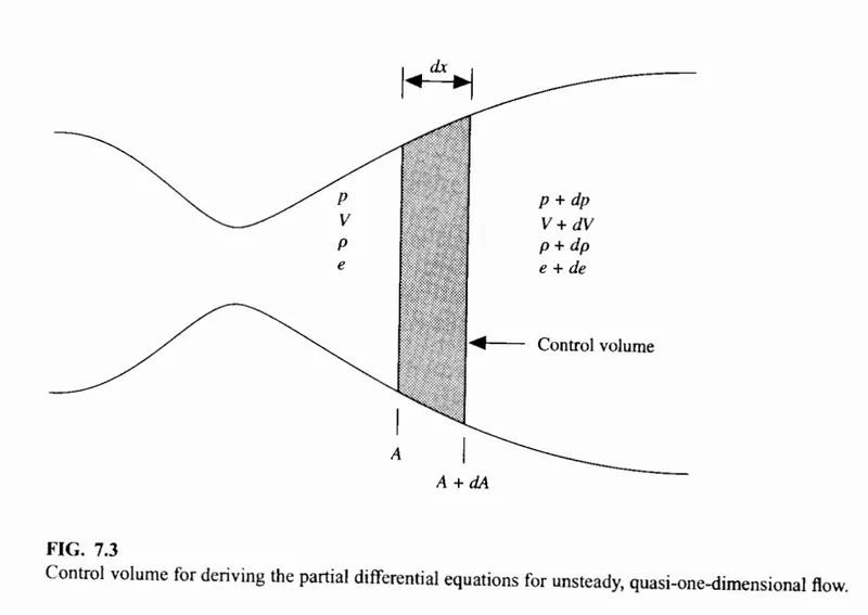
We assume the small control volume of nozzle along the length of nozzle as x dirextion, and its C/A is A consider the flow properties are constant through the nozzle inlet/outlet condition. In reality the flow varies is two spaces i.e(x-y direction), but we assume the flow only in one direction as in consider a x direction along nozzle lenght in that the properties of the flow field are constant across any given C/A such are called as Quasi-One-dimensional flow.

The governing eqaution of Continuity, Momentum and Energy equation in terms of non dimensional variable for this quasi one dimensional steady and isentropic flow can be expressed as for

Non-Conservative Form

1. Contnuity Equation:- `(delrho')/(dt') = -rho'(delV')/(dx')-rho'.V'(del(logA'))/(delx')-V'(delrho')/(delx')`
2. Momentum Equation:- `(delV')/(dt') = -V'(delV')/(dx')-1/(gamma).((delT')/(delx')+(T')/(rho')(delrho')/(delx'))`
3. Energy Equation :-`(delT')/(dt') = -V'(delT')/(dx')-(gamma-1)*T'[(delV')/(delx')+V'(del(logA'))/(delx')]`

Initial Condition

`rho = 1-0.3146x`

`t = 1-0.2314x`

`A = 1+2.2(x-1.5)^2`

Boundary condition

Inlet

`V(1) = 2*V(2)-V(3)`

Outlet

`V(n)=2*V(n-1)-V(n-2)`

`rho(n)=2*rho(n-1)-rho(n-2)`

`t(n)=2*t(n-1)-t(n-2)`

Conservative Form

1. Continuity Equation:- `(del(rho'A'))/(dt')+(del(rho'A'V'))/(dx') = 0`
2. Momentum Equation:- `(del(rho'A'V'))/(dt')+(del[rho'A'V'^2+(1/gamma)rho'A'])/(delx')=1/(gamma)rho'(delA')/(delx')`
3. Energy Equation:-`(del[rho'((e')/(gamma-1)+gamma/2V'^2)A'])/(delt')+(del[rho'((e')/(gamma-1)+gamma/2V'^2)V'A'+rho'A'V'])/(delx')=0`

The above equation can be simplified into following equations.

• `U_1 = rho'A'`
• `U_2 = rho'A'V'`
• `U_3 = rho'(T'1/(gamma-1)+(gamma)/2V'^2)A'`
• `F_1 = rho'A'V'`
• `F_1 = rho'A'V'^2+1/(gamma)rho'A'`
• `F_3 = rho'(T'1/(gamma-1)+(gamma)/2V'^2)A'V'+rho'A'V'`
• `J_2 = 1/(gamma)rho'(dA')/(dx')`

where U1,U2,U3 are solution vector and F1,F2,F3 are the flux vector and J2 are the source term

Substituting the above term in the governing equation

• `(dU_1)/dt' = -(dF_1)/(dx')`
• `(dU_2)/dt' =J_2 -(dF_2)/(dx')`
• `(dU_3)/dt' = -(dF_3)/(dx')`

Initial Condition

`rho = 1-0.3146x`

`t = 1-0.2314x`

`A = 1+2.2(x-1.5)^2`

Boundary condition

Inlet

`V(1) = 2*V(2)-V(3)`

Outlet

`V(n)=2*V(n-1)-V(n-2)`

`rho(n)=2*rho(n-1)-rho(n-2)`

`t(n)=2*t(n-1)-t(n-2)`

Discretization using Macormak Method

Steps in Maccormac Method

• Predictor Method

`(df')/dt_p`

• Solution Updates

`f' = f_(old)+((df)/(dt_p))*Deltat`

• Corrector Method

`(df')/dt_c`

• Calculating Average Value

`((df)/(dt))_(avg) = 0.5*((df')/(dt_p)+(df')/(dt_c))`

• Final Solution Update

`f = f_(old)+((df)/(dt))_(avg)*Deltat`

The main Program of of Non conservative and conservative form

clear
close all
clc

n = 31;
x = linspace(0,3,n);
dx = x(2)-x(1);
tol = 1e-2;
m_analytical = 0.579*ones(1,n);
[m_nc]=Non_conservative_1(n);
[m_c]=Conservative_1(n);

figure(5)
plot(x,m_nc,'b','linewidth',2)
hold on
plot(x,m_c,'r','linewidth',2)
hold on
plot(x,m_analytical,'g','linewidth',2)
title('X Length of Nozzle vs mass flow rate')
xlabel('X Length of Nozzle')
ylabel('Mass Flow rate')
legend({'Non-Conservative', 'Conservative', 'analytical'})

Non-Conservative form of function program

function [m_nc]=Non_conservative_1(n)
  tic
  % Inputes
%   n=31;
  x=linspace(0,3,n);
  dx=x(2)-x(1);
  gamma=1.4;

 % Calculation of initial profile
  rho = 1-0.3146*x;
  t = 1-0.2314*x;
  v = (0.1+1.09*x).*t.^0.5;

 % Area
  a=1+2.2*(x-1.5).^2;

 % Specify throat
  throat=(n+1)/2;
  m_analytical = 0.579*ones(1,n);
  C=0.5;

 % Time step
  nt=1400;
  nt_step=linspace(1,nt,nt);
for p=1:n
    dt_a(p)=C*dx/(t(p)^0.5+v(p));
end
  dt = min(dt_a);

 % Outer time loop
  iter =1;

for k=1:1400
    rho_old = rho;
    v_old = v;
    t_old = t;
    
    
    % Predictor Step
       
  for j = 2:n-1
        dvdx = (v(j+1) -  v(j))/dx;
        drhodx = (rho(j+1) -  rho(j))/dx;
        dtdx  = (t(j+1) - t(j))/dx;
        dlogadx = (log(a(j+1)) - log(a(j)))/dx;
        
        % continuity equation
        drhodt_p(j) = -rho(j)*dvdx - rho(j)*v(j)*dlogadx - v(j)*drhodx;
        
        % Momentum equation
        dvdt_p(j) = -v(j)*dvdx -(1/gamma)*(dtdx  + (t(j)/rho(j))*drhodx);
        
        % Energy Equation
        dtdt_p(j) = -v(j)*dtdx - (gamma-1)*t(j)*(dvdx + v(j)*dlogadx);
        
        
        % Solution Update
           rho(j) = rho(j) + drhodt_p(j)*dt;     % check the sign here.....
           v(j) = v(j) + dvdt_p(j)*dt;
           t(j) = t(j) + dtdt_p(j)*dt;
     
        
        
  end
  
  
  % Corrector Method
  
  
  for j = 2:n-1
        dvdx = (v(j) -  v(j-1))/dx;
        drhodx = (rho(j) -  rho(j-1))/dx;
        dtdx  = (t(j) - t(j-1))/dx;
        dlogadx = (log(a(j)) - log(a(j-1)))/dx;
        
        % continuity equation
        drhodt_c(j) = -rho(j)*dvdx - rho(j)*v(j)*dlogadx - v(j)*drhodx;
        
        % Momentum equation
        dvdt_c(j) = -v(j)*dvdx -(1/gamma)*(dtdx  + (t(j)/rho(j))*drhodx);
        
        % Energy Equation
        dtdt_c(j) = -v(j)*dtdx - (gamma-1)*t(j)*(dvdx + v(j)*dlogadx);
 
  end
  

 % Compute avg time derivative
   drhodt_avg = 0.5*(drhodt_p + drhodt_c);
   dvdt_avg = 0.5*(dvdt_p + dvdt_c);
   dtdt_avg = 0.5*(dtdt_p + dtdt_c);

for i=2:n-1
    rho(i)=rho_old(i)+drhodt_avg(i)*dt;
    v(i)= v_old(i)+dvdt_avg(i)*dt;
    t(i) = t_old(i)+dtdt_avg(i)*dt;

end

   M = v./t.^0.5;
   m_nc = rho.*a.*v;
   m_nct(k,:)=rho.*a.*v;
   iter = iter+1;

  % Applying boundary conditions
  % Inlet
  v(1)=2*v(2)-v(3);
  % Outlet
  v(n)=2*v(n-1)-v(n-2);
  rho(n)=2*rho(n-1)-rho(n-2);
  t(n)=2*t(n-1)-t(n-2);
end
 
figure(1)
 subplot(4,1,1)
 plot(x,rho,'b','linewidth',2)
 xlabel('length of nozzle')
 ylabel('density ratio')
 title('Non-Conservative Form')
 subtitle(sprintf('No of timestep=%d, No of iteration to steady state =%d',k,iter))

 subplot(4,1,2)
 plot(x,v,'g','linewidth',2)
 xlabel('length of nozzle')
 ylabel('velocity ratio')


 subplot(4,1,3)
 plot(x,t,'r','linewidth',2)
 xlabel('length of nozzle')
 ylabel('temp ratio')


 subplot(4,1,4)
 plot(x,M,'black','linewidth',2)
 xlabel('length of nozzle')
 ylabel('Mach Number')


figure(2)
 plot(x,m_nct(50,:),x,m_nct(100,:),x,m_nct(200,:),x,m_nct(300,:),x,m_nct(700,:),x,m_analytical,'linewidth',2)
 xlabel('Non-dimensional distance x')
 ylabel('Non Dimensional mass flow rate')
 title('Variation of mass flow rate(Non-conservative)')
 legend({'50dt','100dt','200dt','300dt','700dt','analytical'})
time_nc = toc;
 fprintf('time of simulation for nonconservative=%gsn,time_nc');
end

Conservative form of function Program

function [m_c]=Conservative_1(n)
% Inputes
tic
% n=31;
x = linspace(0,3,n);
dx = x(2)-x(1);
gamma = 1.4;
throat = (n+1)/2;
m_analytical = 0.579*ones(1,n);

% CalculationInitial Profile
for q=1:n
    if ((x(q)>=0) && (x(q)<=0.5))
        rho(q)=1;
        t(q)=1;
    elseif ((x(q)<1.5) && (x(q)>0.5))
        rho(q) = 1-0.366*(x(q)-0.5);
        t(q) = 1-0.167*(x(q)-0.5);
    elseif ((x(q)>=1.5) && (x(q)<=3.5))
        rho(q) = 0.634-0.3879*(x(q)-1.5);
        t(q) = 0.833-0.3507*(x(q)-1.5);
    end
end

% Area
  a = 1+2.2*(x-1.5).^2;
  v = 0.59./(rho.*a);
  U1 = rho.*a;
  U2= rho.*a.*v;
  U3= rho.*(t/(gamma-1)+(gamma/2)*v.^2).*a;
 
 % Time step

  nt = 1400;
  nt_step = linspace(1,nt,nt);
  C= 0.5;
 for p=1:n
    dt_a(p)=C*dx/(t(p)^0.5+v(p));
end
    dt = min(dt_a);
  
   % Outer Time Loop
     iter =1;
   for k=1:nt
       U1_old = U1;
       U2_old = U2;
       U3_old = U3;
       F1 = U2;
       F2 = (U2.^2)./U1 + ((gamma-1)/gamma)*(U3-(gamma/2)*(U2.^2)./U1);
       F3 = (gamma*U2.*U3)./U1-((gamma*(gamma-1)/2)*(U2.^3)./U1.^2);
      
       % Predictor method
    for j = 2:n-1
        J2(j) = (1/gamma)*rho(j)*t(j)*(a(j+1)-a(j))/dx;
       
        % Continuity equation
        dU1dt_p(j) = -(F1(j+1)-F1(j))/dx;

        % Momentum Equation
        dU2dt_p(j) = J2(j) - (F2(j+1) - F2(j))/dx;

        % Energy Equation 
        dU3dt_p(j) = -(F3(j+1) - F3(j))/dx;


        % Solution Update
        U1(j) = U1(j) + dU1dt_p(j)*dt;
        U2(j) = U2(j) + dU2dt_p(j)*dt;
        U3(j) = U3(j) + dU3dt_p(j)*dt;

    end
    
    rho = U1./a;
    v = U2./U1;
    t = (gamma-1)*((U3./U1)-(gamma/2)*v.^2);
    F1=U2;
    F2 = (U2.^2)./U1 + ((gamma-1)/gamma)*(U3-(gamma/2)*(U2.^2)./U1);
    F3 = (gamma*U2.*U3)./U1-((gamma*(gamma-1)/2)*(U2.^3)./U1.^2);
      
       % Corrector method
    for j = 2:n-1
        J2(j) = (1/gamma)*rho(j)*t(j)*(a(j)-a(j-1))/dx;
       
        % Continuity equation
        dU1dt_c(j) = -(F1(j) - F1(j-1))/dx;

        % Momentum Equation
        dU2dt_c(j) = J2(j) - (F2(j) - F2(j-1))/dx;

        % Energy Equation 
        dU3dt_c(j) = - (F3(j) - F3(j-1))/dx;

    end

       % Avg time derivative

        dU1dt = 0.5*(dU1dt_p + dU1dt_c);
        dU2dt = 0.5*(dU2dt_p + dU2dt_c);
        dU3dt = 0.5*(dU3dt_p + dU3dt_c);

       % Final Updated Solution

       for i = 2:n-1 
           U1(i) = U1_old(i) + dU1dt(i)*dt;
           U2(i) = U2_old(i) + dU2dt(i)*dt;
           U3(i) = U3_old(i) + dU3dt(i)*dt;
       end

       % Boundary Condition

       % Inpute

       U1(1) = rho(1).*a(1);
       U2(1) = 2*U2(2) - U2(3);
       v(1) = U2(1)/(rho(1)*a(1));
       U3(1) = U1(1)*(t(1)/(gamma-1)+(gamma/2)*v(1)^2);

       % Outlet

       U1(n) = 2*U1(n-1) - U1(n-2);
       U2(n) = 2*U2(n-1) - U2(n-2);
       U3(n) = 2*U3(n-1) - U3(n-2);

       % Updating Values

       rho = U1./a;
       v = U2./U1;
       t = (gamma-1)*((U3./U1)-(gamma/2)*v.^2);
       M = v./t.^0.5;
       m_c = rho.*a.*v;
       m_nc(k,:) = rho.*a.*v;

       iter = iter+1;

   end

% Plotting Graph
 figure(3)
  subplot(4,1,1)
  plot(x,rho,'linewidth',2)

   xlabel('length of nozzle')
   ylabel('density ratio')
   title('Conservative Form')
   subtitle(sprintf('No of timestep=%d, No of iteration to steady state =%d',k,iter))

 subplot(4,1,2)
 plot(x,v,'g','linewidth',2)
  
 xlabel('length of nozzle')
 ylabel('velocity ratio')


 subplot(4,1,3)
 plot(x,t,'r','linewidth',2)
 xlabel('length of nozzle')
 ylabel('temp ratio')


 subplot(4,1,4)
 plot(x,M,'black','linewidth',2)
 xlabel('length of nozzle')
 ylabel('Mach Number')

 figure(4)
 plot(x,m_nc(50,:),x,m_nc(100,:),x,m_nc(200,:),x,m_nc(300,:),x,m_nc(700,:),x,m_analytical,'linewidth',2)
 xlabel('Non-dimensional distance x')
 ylabel('Non Dimensional mass flow rate')
 title('Variation of mass flow rate(conservative)')
 legend({'50dt','100dt','200dt','300dt','700dt','analytical'})
time_nc = toc;
 fprintf('time of simulation for conservative=%gsn,time_nc');
end

Result:- The profile of Non-Conservative form and Conservative form

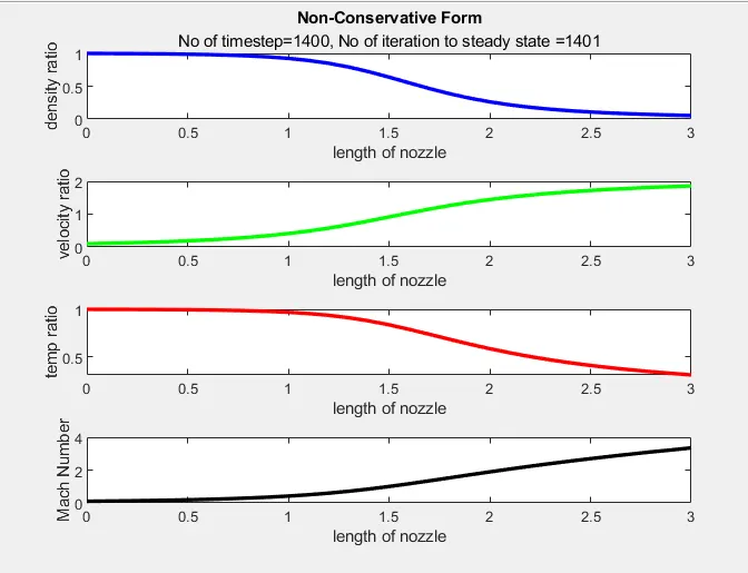
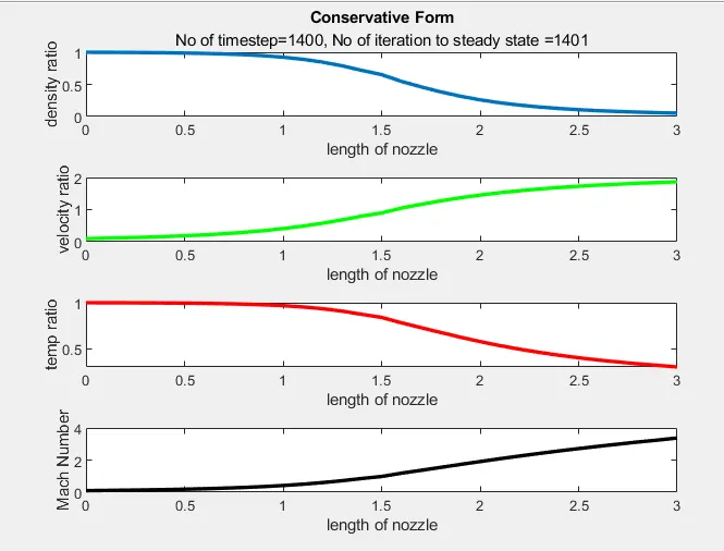
Variation of Mass flow rate at different time steps Non-Conservative & Conservative form

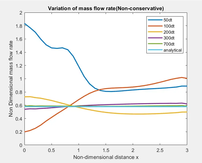
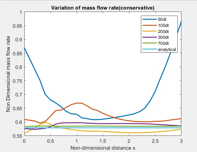
Through the above two graph it shows the time step analyse in different time steps. we observe at 700time step the result comes steady state near about analytical solution. there fore the steady state achieved.

Comparision between Non-Conservative, Conservative and Analytical form.

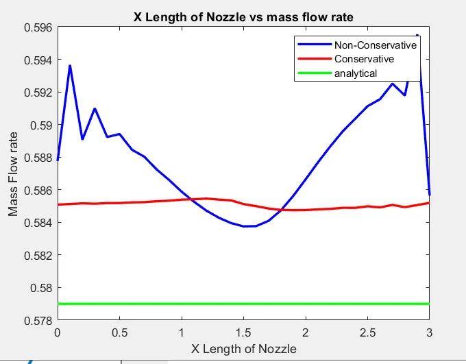
from the above we can see the conservative form of graph show better result as comparative Non conservative steay at analytical form.

Grid dependence test at Non-conservative form

	rho_throat	V_throat	t_throat	M_throat
n=31	0.6387	0.9140	0.8365	0.9994
n=61	0.6377	0.9138	0.8354	0.9998

Grid dependence test at Conservative form

	rho_throat	V_throat	t_throat	M_throat
n=31	0.6524	0.8969	0.8410	0.9780
n=61	0.6391	0.9121	0.8355	0.9979

From the above gride notation we observe small changes at throat in Density, Velocity, Energy and Mach no. at grid 31 & 61. the solution hase not change.