Week 5.1 - Mid term project - Solving the steady and unsteady 2D heat conduction problem
Solving the Steady and Unsteady 2D heat conduction by following steps.
- Staedy state heat conduction by Explicit Method.
- Unsteady state heat condution by Explicit and Implicit Method.
This Explicit and Implicit transient form finding by using Jacobi, Gauss Seidel & SOR Method.
Objective:
- To write the code in matlab to solve 2D heat conduction equation in steady state for given B.C. by using Iterative methods.
- To write the code in matlab to solve 2D heat conduction equation in transient state in explicit method.
- To write the code in matla to solve 2D heat conduction euation in transient state in implicit method, by using Iterative methods.
So we know 2D steady state heat conduction equation as,
`(del^2T)/(delx^2)+(del^2T)/(dely^2)=0`----(1)
So, the B.C. for all four sides our domain are defined initially. we need to solve the temp. for all other points in the domain.
GIVEN DATA
Top Boundary = 600 K
Bottom Boundary = 900 K
Left Boundary = 400 K
Right Boundary = 800 K
The B.C. are defined on all sides we can use the Central difference scheme that take value from all four sides.
The equation 1 differe in central difference form as bellow
`T_(i,j)=(delx^2*dely^2)/(2(delx^2+dely^2))*((T_(i-1,j)+T_(i+1,j))/(delx^2)+(T_(i,j-1)+T_(i,j+1))/(dely^2))`-----(2)
The above equation solve by different iterative technique.
- Jacobi Method
We use following equation to solve for the temp in an iterative loop until the error value i.e. absolute difference error is 1e-4.
`T_(i,j)=(delx^2*dely^2)/(2(delx^2+dely^2))*((T_(old_(i-1,j))+T_(old_(i+1,j)))/(delx^2)+(T_(old_(i,j-1))+T_(old_(i,j+1)))/(dely^2))`----(3)`
'T_old' referece to previous temp at perticular point.
- Gauss Seidel Method
We use following equation to solve for the temp in an iterative loop until the error value.
`T_(i,j)=(delx^2*dely^2)/(2(delx^2+dely^2))*((T_(i-1,j)+T_(old_(i+1,j)))/(delx^2)+(T_(i,j-1)+T_(old_(i,j+1)))/(dely^2))`----(4)`
- Successive Over Relaxation Method
We use following equation to solve for the temp in an iterative loop until the error value is acceptable.
`T_(i,j)=T_(old_(i,j))*(1-omega)+(omega*T_(gs))`----(4)
`where, T_(gs)`=Temp. from Gauss Seidel
`omega`=over relaxation factor
Matlab code for 2D steady state heat conduction.
clear
close all
clc
nx=20;
ny=nx;
x=linspace(0,1,nx);
y=linspace(0,1,ny);
dx=x(2)-x(1);
dy=y(2)-y(1);
T=100*ones(nx,ny);
T(:,1)=400;
T(:,nx)=800;
T(1,:)=900;
T(ny,:)=600;
% Boundary conditions
T_L=400;
T_R=800;
T_B=900;
T_T=600;
% copying of T
% T_initial=T;
T_old=T;
% T1=T1;
% T2=T1;
k1=0.5*(dy^2/(dx^2+dy^2));
k2=0.5*(dx^2/(dx^2+dy^2));

tol=1e-4;
iterative_solver=3;
error=1;
jacobi_iter=1;
% % Jacobi Method
if iterative_solver ==1
    tic
    while(error > tol)
    for i=2:nx-1
      for j=2:ny-1
        T(i,j)=k1*(T_old(i-1,j)+T_old(i+1,j))+k2*(T_old(i,j-1)+T_old(i,j+1));
      end
    end
    time=toc;
    error=max(max(abs(T_old-T)));
    T_old=T;
    jacobi_iter=jacobi_iter+1;
    [c,h]=contourf(x,y,T);
    clabel(c,h)
    colorbar
    colormap(jet)
%     ax=gca;
%     ax.XDir='reverse';
    xlabel('x axis')
    ylabel('T')
    title_text=sprintf('iteration number=%d',jacobi_iter);
    title({'Steady state Temprature profile';['Iteration method =',num2str(iterative_solver)];['No.of iteration=',num2str(jacobi_iter)];['Simulation Time=',num2str(time),'s']});
    pause(0.03)
    grid on
    end
end

% % % GS Method
% T_old =T;
if iterative_solver==2
    tic
    gs_iter=2;
    while(error > tol)
    for i=2:nx-1
      for  j=2:ny-1
        T(i,j)=k1*(T(i-1,j)+T_old(i+1,j))+k2*(T(i,j-1)+T_old(i,j+1));
      end
    end
    time=toc;
    error=max(max(abs(T_old-T)));
    T_old=T;
    gs_iter=gs_iter+1;
    [c,h]=contourf(x,y,T);
   clabel(c,h)
    colorbar
    colormap(jet)
%     ax=gca;
%     ax.XDir='reverse';
    xlabel('x axis')
    ylabel('T')
    title_text=sprintf('iteration number=%d',gs_iter);
    title({'Steady state Temprature profile';['Iteration method =',num2str(iterative_solver)];['No.of iteration=',num2str(gs_iter)];['Simulation Time=',num2str(time),'s']});
    pause(0.03)
    grid on
    end
end

% % % SOR Method
if iterative_solver==3
    omega=1.5;
    tic
    sor_iter=3;
    while(error > tol)
    for i=2:nx-1
      for  j=2:ny-1
        T(i,j)=k1*(T(i-1,j)+T_old(i+1,j))+k2*(T(i,j-1)+T_old(i,j+1));
        T(i,j) = T_old(i,j)*(1-omega)+(T(i,j)*omega);
      end
    end
    time=toc;
    error=max(max(abs(T_old-T)));
    T_old=T;
    sor_iter=sor_iter+1;
   [c,h]=contourf(x,y,T);
   clabel(c,h)
    colorbar
    colormap(jet)
%     ax=gca;
%     ax.XDir='reverse';
    xlabel('x axis')
    ylabel('T')
    title_text=sprintf('iteration number=%d',sor_iter);
    title({'Steady state Temprature profile';['Iteration method =',num2str(iterative_solver)];['No.of iteration=',num2str(sor_iter)];['Simulation Time=',num2str(time),'s']});
    pause(0.03)
    grid on
    end

end
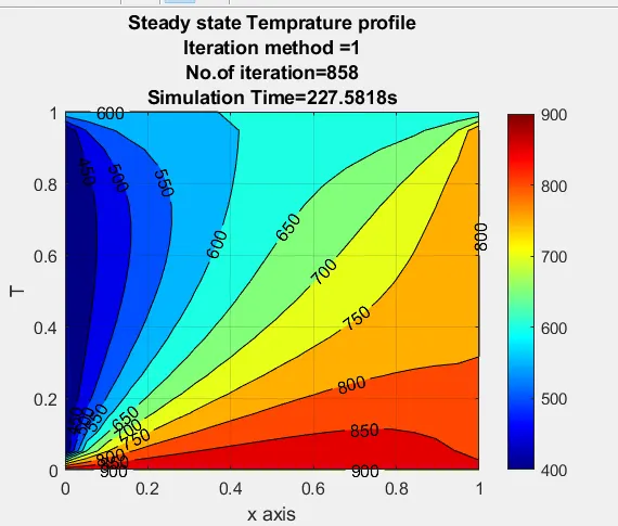
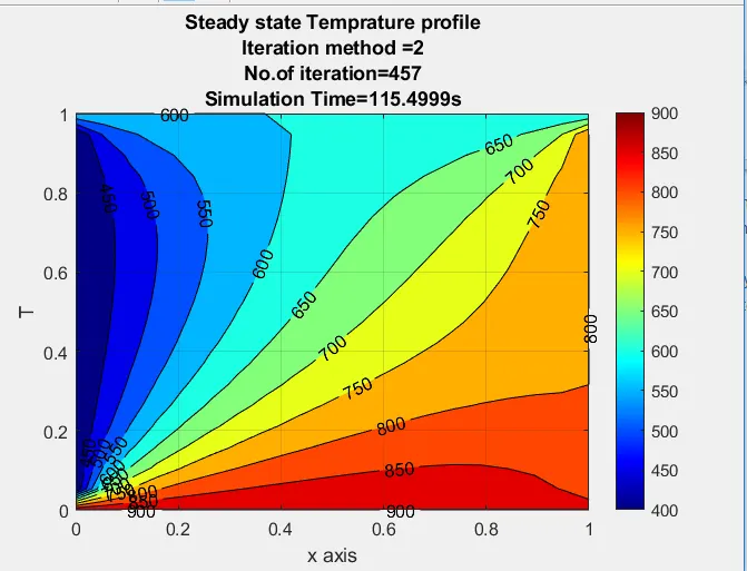
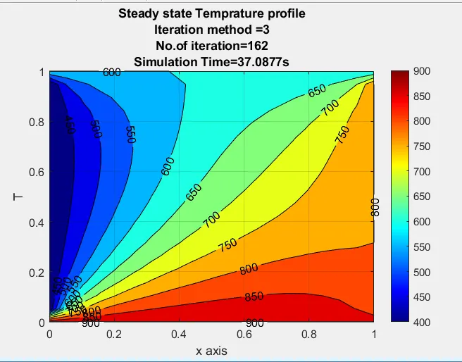
OUTPUT:
- Matlab code of 2D heat conduction for explicit method.
clear
close all
clc
% Parameter
dt=0.0001;
t=0.4;
nt=t/dt;
alpha=1.2;

nx=10;
ny=nx;
x=linspace(0,1,nx);
y=linspace(0,1,ny);
dx=x(2)-x(1);
dy=y(2)-y(1);
T=100*ones(nx,ny);
CFL=alpha*dt*(1/dx^2)+(1/dy^2);
T(:,1)=400;
T(:,nx)=800;
T(1,:)=900;
T(ny,:)=600;
% Boundary conditions
T_L=400;
T_R=800;
T_B=900;
T_T=600;

T_old=T;

k1=alpha*(dt/dx^2);
k2=alpha*(dt/dy^2);

% tol=1e-4;
iterative_solver=0;
% % error=1;
jacobi_iter=0;
% % Jacobi Method
    tic
 % Time loop
 for k=1:nt
     % space loop
    for i=2:nx-1
      for j=2:ny-1
         T(i,j)=T_old(i,j)+k1*(T_old(i-1,j)-2*T_old(i,j)+T_old(i+1,j))+k2*(T_old(i,j-1)-2*T_old(i,j)+T_old(i,j+1));
      end
    end

%     error=max(max(abs(T_old-T)));
    T_old=T;
%     jacobi_iter=jacobi_iter+1;
 end
  time=toc;
  % plotting temprature contour on x and y axes
    [c,h]=contourf(x,y,T);
   clabel(c,h)
    colorbar
    colormap(jet)
%     ax=gca;
%     ax.XDir='reverse';
    xlabel('x axis')
    ylabel('T')
    title_text=sprintf('iteration number=%d',jacobi_iter);
    title({'Transient state Explicit Temprature profile';['Iteration method =',num2str(iterative_solver)];['No.of iteration=',num2str(jacobi_iter)];['Simulation Time=',num2str(time),'s']});
    pause(0.03)
    grid on
OUTPUT
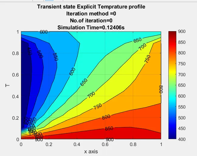
Matlab code of 2D heat conduction for Implicit Method
clear
close all
clc
% Parameter
dt=0.001;
t=0.2;
nt=t/dt;
alpha=1.4;

nx=10;
ny=nx;
x=linspace(0,1,nx);
y=linspace(0,1,ny);
dx=x(2)-x(1);
dy=y(2)-y(1);
T=100*ones(nx,ny);
CFL=alpha*dt*((1/dx^2)+(1/dy^2));
T(:,1)=400;
T(:,nx)=800;
T(1,:)=900;
T(ny,:)=600;
% Boundary conditions
T_L=400;
T_R=800;
T_B=900;
T_T=600;

T_old=T;
T_prev=T;

k1=alpha*(dt/dx^2);
k2=alpha*(dt/dy^2);

 tol=1e-4;
iterative_solver=3;

% jacobi_iter=1;
%  Jacobi Method
if iterative_solver==1
    tic
    iter=1;
 % Time loop
 for k=1:nt
     error=1;
     while( error > tol)
     % space loop
    for i=2:nx-1
      for j=2:ny-1
        term1=1/(1+2*k1+2*k2);
        term2=k1*term1;
        term3=k2*term1;
        H=T_old(i-1,j)+T_old(i+1,j);
        V=T_old(i,j-1)+T_old(i,j+1);
        T(i,j)=T_prev(i,j)*term1+(H*term2)+(V*term3);
      end
    end
    time=toc;
    error=max(max(abs(T-T_old)));
    T_old=T;
    iter=iter+1;
     end
     T_prev=T;
  % plotting temprature contour on x and y axes
    [c,h]=contourf(x,y,T);
   clabel(c,h)
    colorbar
    colormap(jet)
%     ax=gca;
%     ax.XDir='reverse';
    xlabel('x axis');
    ylabel('T');
    title_text=sprintf('iteration number=%d',iter);
    title({'Transient State Implicit profile';['Iteration method =',num2str(iterative_solver)];['No.of iteration=',num2str(iter)];['Time=',num2str(t),'s'];['CFL=',num2str(CFL)];['Simulation Time=',num2str(time),'s']});
    pause(0.03);
    grid on

 end
end

% % % GS Method
if iterative_solver==2
    tic
    iter=2;
    for k=1:nt
        error=1;
    while(error > tol)
    for i=2:nx-1
      for  j=2:ny-1
        term1=1/(1+2*k1+2*k2);
        term2=k1*term1;
        term3=k2*term1;
        H=T(i-1,j)+T_old(i+1,j);
        V=T(i,j-1)+T_old(i,j+1);
        T(i,j)=T_prev(i,j)*term1+(H*term2)+(V*term3);
      end
    end
    time=toc;
    error=max(max(abs(T-T_old)));
    T_old=T;
    iter=iter+1;
    end
    T_prev=T;
    [c,h]=contourf(x,y,T);
   clabel(c,h)
    colorbar
    colormap(jet)
%     ax=gca;
%     ax.XDir='reverse';
    xlabel('x axis')
    ylabel('T')
    title_text=sprintf('iteration number=%d',iter);
    title({'Transient State Implicit profile';['Iteration method =',num2str(iterative_solver)];['No.of iteration=',num2str(iter)];['Time=',num2str(t),'s'];['CFL=',num2str(CFL)];['Simulation Time=',num2str(time),'s']});
    pause(0.03)
    grid on
    end
end

% % % SOR Method
if iterative_solver==3
    omega=1.1;
    tic
    iter=3;
    for k=1:nt
        error=1;
    while(error > tol)
    for i=2:nx-1
      for  j=2:ny-1
        term1=1/(1+2*k1+2*k2);
        term2=k1*term1;
        term3=k2*term1;
        H=T(i-1,j)+T_old(i+1,j);
        V=T(i,j-1)+T_old(i,j+1);
        T(i,j)=T_prev(i,j)*term1+(H*term2)+(V*term3);
        T(i,j) = T_old(i,j)*(1-omega)+(T(i,j)*omega);
      end
    end
    time=toc;
    error=max(max(abs(T_old-T)));
    T_old=T;
    iter=iter+1;
    end
    T_prev=T;
   [c,h]=contourf(x,y,T);
   clabel(c,h)
    colorbar
    colormap(jet)
%     ax=gca;
%     ax.XDir='reverse';
    xlabel('x axis')
    ylabel('T')
    title_text=sprintf('iteration number=%d',iter);
    title({'Transient state Implicit profile';['Iteration method =',num2str(iterative_solver)];['No.of iteration=',num2str(iter)];['Time=',num2str(t),'s'];['CFL=',num2str(CFL)];['Simulation Time=',num2str(time),'s']});
    pause(0.03)
    grid on
    end
end
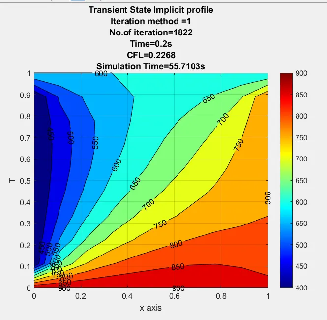
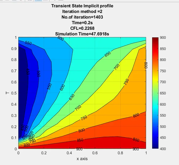
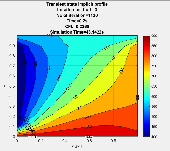
Output
Conclusion:
The Successive_Over_Relaxation _Method is more accure and less number of iteration than Gauss_Seidel & Jacobi_Method.
i.e. Jacobi<Gauss_Seidel<Successive_Over_Relaxation.
In this project we study the steady method and unsteady method in that SOR method is approches most efficient. And fastest steady is observed SOR method & unsteady state it also Implicit SOR method.