Week 3.5 - Deriving 4th order approximation of a 2nd order derivative using Taylor Table method
###Taylor's Table
## The fourth order approximation of Second order derivative.
## Skewed Approximation,
##skewed right sided difference
# No.of nodes = P+Q,(where as P=Order of derivative is =2, Q=order of approximation =4);
# No. of nodes =2+4=6; (So, toltal 6 nodes required for accurate skewed right sided differences);
%right_sided_skewed_difference= (a*f(i)+b*f(i+1)+c*f(i+2)+d*f(i+3)+e*f(i+4)+g*f(i+5))/(dx)^2
%1 .a+b+c+d+e+g = 0;
%2. b+2*c+3*d+4*e+5*g = 0;
%3. b+4*c+9*d+16*e+25*g = 2;
%4.(b/6)+(8*c/6)+(27*d/6)+(64*e/6)+(125*g/6) = 0;
%5.(b/24)+(16*c/24)+(81*d/24)+(256*e/24)+(625*g/24) = 0;
%6.(b/120)+(32*c/120)+(243*d/120)+(1024*e/120)+(3125*g/120) = 0;
A=[1 1 1 1 1 1; 0 1 2 3 4 5; 0 1/2 2 9/2 16/2 25/2; 0 1/6 8/6 27/6 64/6 125/6;
0 1/24 16/24 81/24 256/24 625/24; 0 1/120 32/120 243/120 1024/120 3125/120];
B=[0;0;1;0;0;0];
X=(A\B);
##Skewed left sided difference
# No.of nodes = P+Q,(where as P=Order of derivative is =2, Q=order of approximation =4);
# No. of nodes =2+4=6; (So, toltal 6 nodes required for accurate skewed left sided differences);
%left_sided_skewed_difference= (a*f(i)+b*f(i-1)+c*f(i-2)+d*f(i-3)+e*f(i-4)+g*f(i-5))/(dx)^2
% g+e+d+c+b+a=0;
% (-5*g)-(4*e)-(3*d)-(2*c)-b=0;
% (25*g/2)+(16*e/2)+(9*d/2)+(4*c/2)+(b/2)=1;
% (-125*g/6)-(64*e/6)-(27*d/6)-(8*c/6)-(b/6)=0;
% (625*g/24)+(256*e/24)+(81*d/24)+(16*c/24)+(b/24)=0;
% (-3125*g/120)-(1024*e/120)-(243*d/120)-(32*c/120)-(b/120)=0;
C=[1 1 1 1 1 1; -5 -4 -3 -2 -1 0; 25/2 16/2 9/2 4/2 1/2 0; -125/6 -64/6 -27/6 -8/6 -1/6 0;
625/24 256/24 81/24 16/24 1/24 0; -3125/120 -1024/120 -243/120 -32/120 -1/120 0];
D=[0;0;1;0;0;0];
Y=(C\D);
##central skewed difference
# No.of nodes = P+Q-1,(where as P=Order of derivative is =2, Q=order of approximation =4);
# No. of nodes =2+4-1=5; (So, toltal 5 nodes required for accurate skewed central differences);
# Central_difference = (a*f(i-2)+b*f(i-1)+c*f(i)+d*f(i+1)+e*f(i+2))/(dx)^2;
% a+b+c+d+e=0;
% (-2*a)-b+0+d+2*e=0;
% (4*a/2)+(b/2)+0+(d/2)+(4*e/2)=1;
% (-8*a/6)-(b/6)0+(d/6)+(8*e/6)=0;
% (16*a/24)+(b/24)+0+(d/24)+(16*e/24)=0;
E=[1 1 1 1 1; -2 -1 0 1 2; 2 0.5 0 0.5 2; -4/3 -1/6 0 1/6 4/3; 2/3 1/24 0 1/24 2/3];
F=[0;0;1;0;0];
z=(E\F);
###Right Sided Skewed approximation Program
function out=right_sided_skewed_approximations_function(x,dx);
% analytical derivative
analytical_derivative =-2*exp(x)*sin(x);
% numerical derivative
%fourth order right sided skewed approximation
a=3.75; b=-12.8333333333333; c=17.8333333333333; d=-13; e=5.083333333333;
g=-0.83333333333;
%right_sided_skewed_difference= (a*f(i)+b*f(i+1)+c*f(i+2)+d*f(i+3)+e*f(i+4)+g*f(i+5))/(dx)^2
right_sided_skewed_difference = (a*(exp(x)*cos(x))+b*(exp(x+dx)*cos(x+dx))+c*(exp(x+2*dx)*cos(x+2*dx))+
d*(exp(x+3*dx)*cos(x+3*dx))+e*(exp(x+4*dx)*cos(x+4*dx))+g*(exp(x+5*dx)*cos(x+5*dx)))/(dx)^2;
%out put
out = abs(right_sided_skewed_difference-analytical_derivative);
endfunction
### Left Sided Skewed approximation Program
function out=left_sided_skewed_approximations_function(x,dx);
% analytical derivative
analytical_derivative =-2*exp(x)*sin(x);
% numerical derivative
%fourth order right sided skewed approximation
a=3.75; b=-12.833333333333; c=17.8333333333333333; d=-13; e=5.083333333333333;
g=-0.8333333333333;
%left_sided_skewed_difference= (a*f(i)+b*f(i-1)+c*f(i-2)+d*f(i-3)+e*f(i-4)+g*f(i-5))/(dx)^2
left_sided_skewed_difference =(g*(exp(x-5*dx)*cos(x-5*dx))+e*(exp(x-4*dx)*cos(x-4*dx))+d*(exp(x-3*dx)*cos(x-3*dx))+
c*(exp(x-2*dx)*cos(x-2*dx))+b*(exp(x-dx)*cos(x-dx))+a*(exp(x)*cos(x)))/(dx)^2;
%out put
out = abs(left_sided_skewed_difference-analytical_derivative);
endfunction
### Central Skewed approximation
function out=central_approximations_function(x,dx);
% analytical derivative
analytical_derivative = -2*exp(x)*sin(x);
% numerical derivative
%fourth order right sided skewed approximation
a=-0.08333333333333333333; b=1.3333333333333333333; c=2.5; d=b; e=a;
# Central_difference = (a*f(i-2)+b*f(i-1)+c*f(i)+d*f(i+1)+e*f(i+2))/(dx)^2;
central_difference = (a*(exp(x-2*dx)*cos(x-2*dx))+b*(exp(x-dx)*cos(x-dx))+c*(exp(x)*cos(x))+
d*(exp(x+dx)*cos(x+dx))+e*(exp(x+2*dx)*cos(x+2*dx)))/(dx)^2;
%out put
out = abs(central_difference-analytical_derivative);
endfunction
### Main program For Loop
clear all
close all
clc
% value of x and dx
x = pi/2;
dx = linspace(pi/4,pi/400,20);
for i=1:length(dx)
right_sided_skewed_error(i)=right_sided_skewed_approximations_function(x,dx(i));
left_sided_skewed_error(i)=left_sided_skewed_approximations_function(x,dx(i));
central_error(i)= central_approximations_function(x,dx(i));
endfor
%plotting in graph dx value against error
figure(1)
hold off
loglog(dx,right_sided_skewed_error,'b-o','linewidth',1.5)
hold on
loglog(dx,left_sided_skewed_error,'r-o','linewidth',1.5)
hold on
loglog(dx,central_error,'g-o','linewidth',1.5)
xlabel('dx')
ylabel('Absolute error')
legend ('right sided error','left sided skewed error','central error')
legend ('right sided error','left sided skewed error','central error','location','northwest')
title('Plotting Graph Between dx and Absolute Error')
@@ OUTPUT:
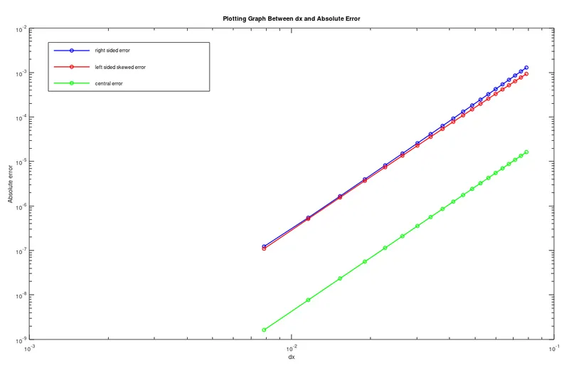
@@ CONCLUSION:The above graph shows Central Difference Approximation Error is less than Left Difference Approximation Error and Right Difference Approximation Error, i.e.(CDAE<LDAE<FDAE).
Thats why more accurate answer Central Difference Approximation used than FDA BDA.