Week 7 - Simulation of a 1D Super-sonic nozzle flow simulation using Macormack Method

Aim : Simulation of a 1D Super-sonic nozzle flow simulation using Macormack Method

Objective :

1)study conservation and non conservation form of governing equations

2) Study Mackormecks technique to solve time variation of primitive variable in 1D supersonic flow through nozzle

3) Derive conservation and non conservation forms of governing equations

4) use forward and backward differencing scheme for discreatization of governing equations

Theory :

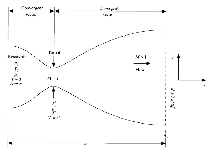
we consider the convergent divergent nozzle as shown in the figure . the flow at the inlet to the nozzle comes from a reservoir where the presure and temperature are denoted by p0 ,T0 .crossectional area of reservoir is very large (`A to infty`) and therefore velocity is really small. Thus, p0 and T0 are the stagnation values or total pressure and total temperature respectively. Theflow expands isentropically to supersomic speed at the nozzle exit ,where the pressure, temperature,velocity and macj number are denoted by pe,Te,Ve an Me. the flow is locally subsonic in convertgent section of the nozzle, sonic at the throat and supersonic at the divergent section. The sonic flow (M=1) at the throat means that local velocity at this location is equal to local speed of sound.

1) Non conservation :

Governing equation:

Contuinity equation :

`(delrho) /(delt) = rho'*(delV')/(delx') - rho'*V'*(del(lnA))/(delx') -V'*(delrho')/(delx')`

Momentum Equation:

`(delV')/(delt') = -V'*(delV')/(delx') - (1/gamma) *((delT')/(delx') + (T')/(rho')*(delrho')/(delx'))`

Energy Equation :

`(delT')/(delt') = -V'*(delT')/(delx') - (gamma-1)*T'*((delV')/(delx') + V'*(del(lnA))/(delx'))`

where ,

`x' = (x/L)`

`V' = V/(a_0)`

`t' = t/(L/(a_0))`

`A' = A/(A^star)`

`a_0` = speed of sound in reservoir

`A_star` = Throat Area

this are all non dimensional quantities.

now solving these equations using Mackormecks technique

Predictors step :

forward diffferencing this above equations

now getting new updated value for primitive variables :

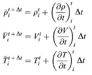
Correctors step :

discreatizing with backward differencing scheme and taking updated values of primitive variables

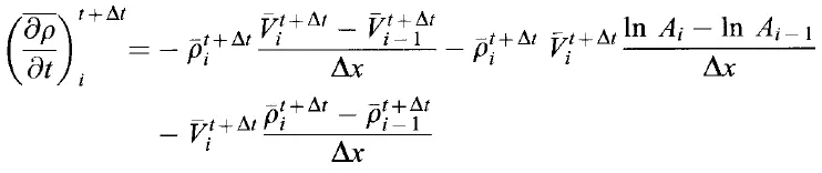
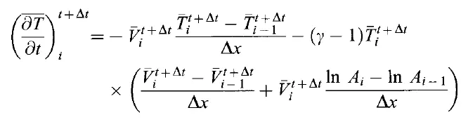
Now Calculating Average time derivative :

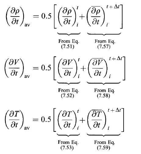
Making Final Solution Update :

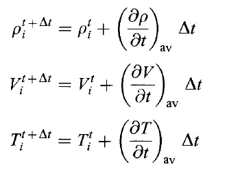
Now repeating this steps with nth no. of time step values untill equations becomes stable

Main Programme :

close all 
clear all 
clc

%% Inputs 
n = 31;
x = linspace(0,3,n);
dx = x(2)-x(1) ;
gamma = 1.4;
CFL =0.5;
nt = 1:1400;

tic ;
%% Non conservation function 
[V_throat_nc,t_throat_nc,rho_throat_nc,mach_throat_nc,p_throat_nc,mass_f_r_throat_nc,mass_flow_rate_nc] = non_conservation(n,x,dx,gamma,CFL);


%% Plotting Primitive Variables at throat 
figure(4) 
subplot(3,1,1) 
plot(nt,V_throat_nc,'linewidth',2,'color','r') ;
ylabel('Velocity')
xlabel('time steps')

subplot(3,1,2) 
plot(nt,rho_throat_nc,'linewidth',2,'color','b') ;
ylabel('Density')
xlabel('time steps')

subplot(3,1,3) 
plot(nt,t_throat_nc,'linewidth',2,'color','g') ;
ylabel('temperature')
xlabel('time steps')

figure(5)
subplot(3,1,1) 
plot(nt,p_throat_nc,'linewidth',2,'color','r') ;
ylabel('pressure')
xlabel('time steps')

subplot(3,1,2) 
plot(nt,mach_throat_nc,'linewidth',2,'color','b') ;
ylabel('Mach Number')
xlabel('time steps')

subplot(3,1,3) 
plot(nt,mass_f_r_throat_nc,'linewidth',2,'color','g') ;
ylabel('mass flow rate')
xlabel('time steps')

time_nc = toc 

tic 
%% Function for Conservation form 
[V_throat_c,t_throat_c,rho_throat_c,mach_throat_c,mass_f_r_throat_c,p_throat_c,mass_flow_rate_c] = Conservation(n,nt,CFL);

%% Plotting Primitive Variables at throat 
figure(9) 
subplot(3,1,1) 
plot(nt,V_throat_c,'linewidth',2,'color','r') ;
ylabel('Velocity')
xlabel('time steps')

subplot(3,1,2) 
plot(nt,rho_throat_c,'linewidth',2,'color','b') ;
ylabel('Density')
xlabel('time steps')

subplot(3,1,3) 
plot(nt,t_throat_c,'linewidth',2,'color','g') ;
ylabel('temperature')
xlabel('time steps')

figure(10)
subplot(3,1,1) 
plot(nt,p_throat_c,'linewidth',2,'color','r') ;
ylabel('pressure')
xlabel('time steps')

subplot(3,1,2) 
plot(nt,mach_throat_c,'linewidth',2,'color','b') ;
ylabel('Mach Number')
xlabel('time steps')

subplot(3,1,3) 
plot(nt,mass_f_r_throat_c,'linewidth',2,'color','g') ;
ylabel('mass flow rate')
xlabel('time steps')

time_c = toc
%% Steady state Mass flow rate comparision 
figure(11)
plot(x,mass_flow_rate_nc,'color','r','linewidth',3);
hold on 
plot(x,mass_flow_rate_c,'color','g','linewidth',3);
xlabel('length of nozzle')
ylabel('mass flow rate')
legend('Non Conservation','Conservation')
title(' Comparison of Normalized mass flow rate distributions of both forms')

Function for solving Non Conservation form of Equation:

function [V_throat_nc,t_throat_nc,rho_throat_nc,mach_throat_nc,p_throat_nc,mass_f_r_throat_nc,mass_flow_rate_nc] = non_conservation(n,x,dx,gamma,CFL)

%% Calculating Initial Profiles 

rho = 1-0.3146.*x ;
t = 1-0.2314*x;  % t = temperature 
V = (0.1 +1.09*x).*t.^0.5 ; 

% Area
a = 1+2.2*(x-1.5).^2 ; 
%time step 
nt = 1400;


%% outer time loop 
% conditions at starting of time step 
t_old = t;
V_old = V;
rho_old = rho;

 % time step size 
for ts =1:n
     a_sound = sqrt(t(ts));
     dt(ts) = CFL*dx/(a_sound +V(ts));
end 
dt = min(dt); 

for k = 1:nt % time loop
    t_old = t ;
    V_old = V;
    rho_old = rho;
    
   
    
    %predictors loop 
    for j = 2:n-1 
        
        dv_dx = (V(j+1) -V(j))./dx;
        drho_dx = (rho(j+1)-rho(j))./dx;
        dt_dx = (t(j+1) -t(j))./dx;
        dloga_dx = (log(a(j+1))-log(a(j)))./dx; 
      
        
        % Contuinity equation 
        drho_dt_p(j) = -rho(j).*dv_dx -rho(j).*V(j).*dloga_dx - V(j).*drho_dx;
        
        % Momentum equation
        dv_dt_p(j) = -V(j).*dv_dx -(1/gamma)*(dt_dx +(t(j)/rho(j)).*drho_dx);
        
        %Energy equation 
        dt_dt_p(j) = -V(j).*dt_dx -(gamma-1).*t(j).*(dv_dx +V(j)*dloga_dx);
        
        %Solution upate 
        
        V(j) = V(j) + dv_dt_p(j).*dt ;
        t(j) = t(j) + dt_dt_p(j).*dt ;
        rho(j) = rho(j) + drho_dt_p(j).*dt;
    
    
    
    %% Correctors loop 
    
        
        dv_dx = (V(j) -V(j-1))./dx;
        drho_dx = (rho(j)-rho(j-1))./dx;
        dt_dx = (t(j) -t(j-1))./dx;
        dloga_dx = (log(a(j))-log(a(j-1)))./dx; 
      
        
        % Contuinity equation 
        drho_dt_c(j) = -rho(j).*dv_dx -rho(j).*V(j).*dloga_dx - V(j).*drho_dx;
        
        % Momentum equation
        dv_dt_c(j) = -V(j).*dv_dx -(1/gamma)*(dt_dx +(t(j)/rho(j))*drho_dx);
        
        %Energy equation 
        dt_dt_c(j) = -V(j).*dt_dx -(gamma-1).*t(j)*(dv_dx +V(j)*dloga_dx);
         
    
    end 
    %% Computing average time derivative 
        
       drho_dt_avg = 0.5.*(drho_dt_p+drho_dt_c);
       dv_dt_avg = 0.5.*(dv_dt_p+dv_dt_c);
       dt_dt_avg = 0.5.*(dt_dt_p + dt_dt_c);
       
       %% Final Solution Update 
       for i =2:n-1 
       rho(i) = rho_old(i) + drho_dt_avg(i).*dt ;
       V(i)   = V_old(i) +dv_dt_avg(i).*dt;
       t(i) = t_old(i) + dt_dt_avg(i).*dt;
       end
       
       %% Apply Boundary Conditions 
       % Inlet Boundary Conitio
       V(1) = 2*V(2) -V(3) ;  
       
       
       %Outlet Bounary Conditions 
       
       V(n) = 2.*V(n-1) -V(n-2) ;
       rho(n) = 2.*rho(n-1) - rho(n-2) ;
       t(n) = 2.*t(n-1) -t(n-2) ;
    
       
 %% Calculating other quantities 
mass_flow_rate_nc = rho.*a.*V;
pressure = rho.*t ;
mach_number = V./((t).^0.5);

   
%% Throat Variables 
V_throat_nc(k) = V(16);
t_throat_nc(k) = t(16);
rho_throat_nc(k) = rho(16);
p_throat_nc(k)  = pressure(16);
mach_throat_nc(k) = mach_number(16);
mass_f_r_throat_nc(k) = mass_flow_rate_nc(16);


% plotting mass flow rate at various time step 

for l = [1,50,100,150,200,700]
    if l==k
        figure(1)
        plot(x,mass_flow_rate_nc)
        hold on 
    elseif k==1400
        plot(x,mass_flow_rate_nc)
    end  
    xlabel('Length of nozzle');
    ylabel('Mass Flow Rate');
    legend('time-step=1','time step=50','time step=100','time step=150','time step=200','time step=700','time step=1400')
    title('Variation of Mass flow rate distribution inside the nozzle at different time steps during the time-marching process');
    
end
    

end

%% Plotting 

ntr = 1:1400;
figure(2)
plot(ntr,V_throat_nc)
hold on 
plot(ntr,t_throat_nc)
plot(ntr,rho_throat_nc)
plot(ntr,p_throat_nc)
plot(ntr,mach_throat_nc)
plot(ntr,mass_f_r_throat_nc)
legend('velocity','temperature','density','pressure','machnumber','mass flow rate')
 ylabel('non dimensionless parameters')  ;
 xlabel('no. of time steps')
 title('Time-wise variation of primitive variables')
 
figure(3)
plot(x,V,'linewidth',2);
hold on 
plot(x,t,'linewidth',2);
plot(x,rho,'linewidth',2);
plot(x,pressure,'linewidth',2);
plot(x,mach_number,'linewidth',2);
plot(x,mass_flow_rate_nc,'linewidth',2);
legend('velocity','temperature','density','pressure','machnumber','mass flow rate')
 ylabel('non dimensionless parameters')  ;
 xlabel('length of nozzle ')
 title('steady state distribution  of primitive variables inside nozzle')
 
 

end

Explanation Of code :

1. define all inputs given and assumed for solving equations take grid value to be 31.
2. Calculating initial values of primitive variables which are given as inputs for solving by mackormecks method
3. specify no. of time steps and area of nozzle
4. calculate size of time step size at each grid spacing by considering CFL number to be 0.5, take minimum value of step size from all values obtained at each grid spacing
5. specify time loop and under time loop specify old values of primitive variables which are to be calculate at previous time step so that we can use this in mackormecks method
6. start the predictors loop, find `(delrho)/(dt) ,(delV')/(delt) ,(delt')/(delt)` at first time step using forward differencing scheme
7. now calculate updated value of `rho',t',V'`
8. Now start correctors loop , solve for updated values of `(delrho)/(dt) ,(delV')/(delt) ,(delt')/(delt)` using backward differencing scheme .
9. Find Average time derivative and update the solution by using average time derivative
10. specify boundary conditions and calculate mass flow rate ,pressure , mach number from primitive variables
11. repeat these steps for nth time steps values untill our solution bcomes stable
12. Plot the time wise and steady state variation of primitive variables inside nozzle
13. plot variation of mass flow rate for various time steps and observe how it changes with time step

Results and plots :

1)Variation of mass flow rate distribution inside the nozzle at different time steps during the time marching process :

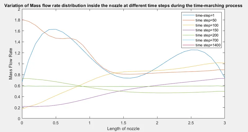
observation : there are fluctions in mass flow rate at lesser time steps because the solution hasnt converged yet ,

after 200 time step value mass flow rate becoming flat and the fluctuations tends to be reducing. after 700 time step value mass flow rate becomes straight , and this

satisfies Contuinity equation throghout the nozzle

2)Time-wise Variation of primitive Variables inside nozzle :

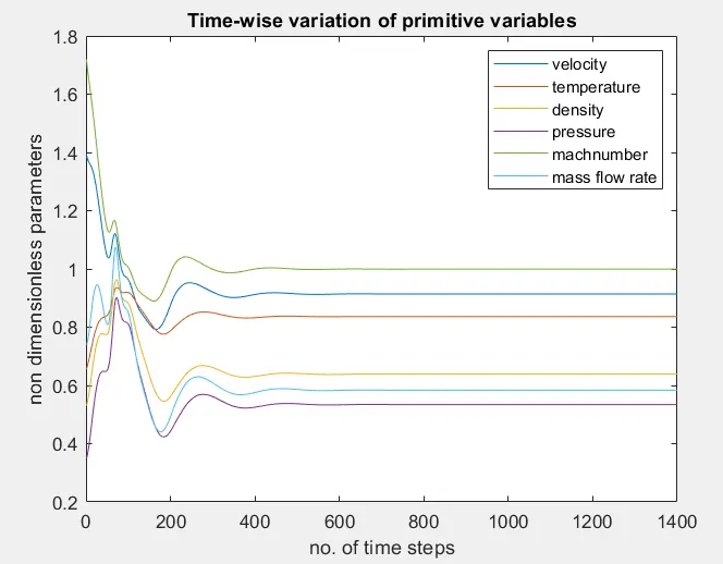
observation : we can see that there are fluctuations in values of primitive variables at intial stages at lesser time steps, this is also known as rubber band effect.

it takes some time marching to acheive orginial value of solution . values of primitive variables becoming straight line after 200 time steps.

3)Steady state Distribution of primitive variables inside nozzle

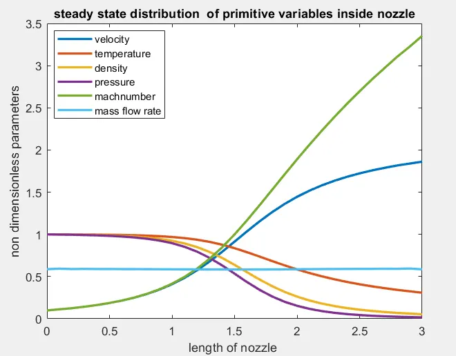
Observation : we can observe that Mach number and velocity increases with length of nozzle. pressure ,density and temperature decreases with increase in length of nozzle.

also we can observe here validation of contuinity equation , i.e. `(rhoVA)1 = (rhoVA)2` , because mass flow rate remaining constant throghout the length of nozzle

5)Variation of primitive variables with time steps :

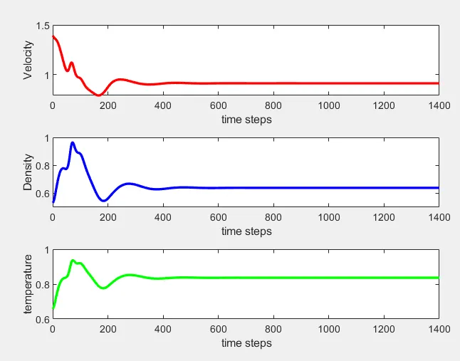
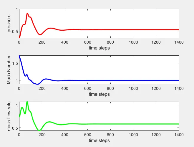
Observation : we can see from above plots variations of primitive variables with time steps, as they are first have more fluctuations and then

with time steps this fluctuation reduced.

Conservation Form :

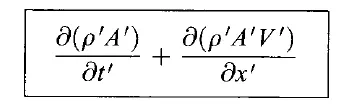
1) Governing Equations :

Contuinity equation :

Momentum Equation :

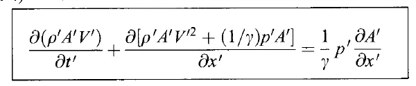
Energy Equation :

`x' = (x/L)`

`V' = V/(a_0)`

`t' = t/(L/(a_0))`

`A' = A/(A^star)`

`a_0` = speed of sound in reservoir

`A_star` = Throat Area

replacing terms in above equation with

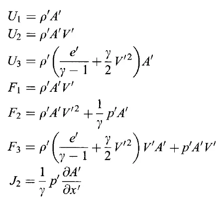
where ,

U1,U2,U3 = solution vector

F1,F2,F3 = Flux terms

J2 = Source term

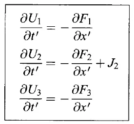
so modified contuinity,momentum and energy equation will be

F1,F2,F3,J2 should be functions of U1,U2,U3 because it is a solution vector and we need to solve for F1,F2,F3 an J2

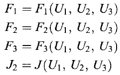
By deriving this equations we get

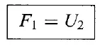
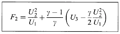
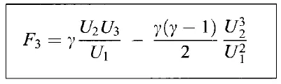
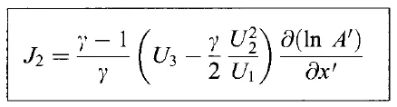
Now solving for these terms using Mackormecks Method which is mentioned above in non conservation section.

Function for Conservation Form :

function[V_throat_c,t_throat_c,rho_throat_c,mach_throat_c,mass_f_r_throat_c,p_throat_c,mass_flow_rate_c] = Conservation(n,nt,CFL)



x = linspace(0,3,n);
dx = x(2)-x(1) ; 
gamma = 1.4;

%% Initial Conditions 

a = 1+2.2*(x-1.5).^2;


%% Initial Conditions 
for i=1:1:length(x)
    
    if(x(i)>=0 && x(i)<=0.5)
        rho(i)=1;
        t(i)=1;
        
    elseif (x(i)>=0.5  && x(i)<=1.5)
          rho(i)=1-0.366*(x(i)-0.5);
          t(i)=1-0.167*(x(i)-0.5);
                
    elseif (x(i)>=1.5  && x(i)<=3)
           rho(i)= 0.634-0.3879*(x(i)-1.5);
           t(i)= 0.833-0.3507*(x(i)-1.5);
        
    end 
end 
    % Solution Vectors 
e = t;
V = 0.59./(rho.*a);
U1= rho.*a;
U2= rho.*a.*V;
U3= rho.*a.*((t./(gamma-1))+(gamma/2).*V.^2);




% Solution Vectors 
%% Time loop 
for tt = 1:1:length(nt) 
 % Storing Initial Values 
    U1_old = U1;
    U2_old = U2;
    U3_old = U3;
    
    dt =min((CFL.*dx)./(t.^(0.5)+V));
   
    F1= U2;
    F2= ((U2.^2)./U1 )+ ((gamma-1)/gamma).*(U3-((gamma/2) * (U2.^2)./U1));
    F3= ((gamma*U2.*U3)./U1) - ((gamma*(gamma-1)/2) * (U2.^3)./(U1.^2));
      
    for nx = 2:n-1 
    %% Predictors step 
      % Source term J2
      J2(nx) = (1/gamma)*rho(nx)*t(nx)*((a(nx+1)-a(nx))/dx);  
      % Predictors Step derivative  
      du1dt_p(nx) = -(F1(nx+1)-F1(nx))./dx ;
      du2dt_p(nx) = -(F2(nx+1)-F2(nx))./dx + J2(nx) ;
      du3dt_p(nx) = -(F3(nx+1)-F3(nx))./dx ;
      
      % Solution update 
      U1(nx) = U1_old(nx) + du1dt_p(nx).*dt;
      U2(nx) = U2_old(nx) + du2dt_p(nx).*dt;
      U3(nx) = U3_old(nx) + du3dt_p(nx).*dt;

    end 
    rho =U1./a ;
    V=U2./U1;
    t = (gamma-1).*((U3./U1) - (gamma./2).*(V).^2);
    
    % correctors step 
    % Flux Vector 
    F1= U2;
    F2= ((U2.^2)./U1 )+ ((gamma-1)/gamma).*(U3-((gamma/2) * (U2.^2)./U1));
    F3= ((gamma*U2.*U3)./U1) - ((gamma*(gamma-1)/2) * (U2.^3)./(U1.^2));
    
    
    for j = 2:n-1 
    % Source term J2
    J2(j) = (1/gamma)*rho(j)*t(j)*((a(j)-a(j-1))/dx);
    % Correctors Step derivative  
    du1dt_c(j) = -(F1(j)-F1(j-1))./dx ;
    du2dt_c(j) = -(F2(j)-F2(j-1))./dx + J2(j) ;
    du3dt_c(j) = -(F3(j)-F3(j-1))./dx ;

    end

    % Average time derivative 
    du1dt_avg = 0.5.*(du1dt_p + du1dt_c);
    du2dt_avg = 0.5.*(du2dt_p + du2dt_c);
    du3dt_avg = 0.5.*(du3dt_p + du3dt_c);

    %% Final Solution update 
    for y =2:n-1 
      
        U1(y) = U1_old(y) + du1dt_avg(y).*dt;
        U2(y) = U2_old(y) + du2dt_avg(y).*dt;
        U3(y) = U3_old(y) + du3dt_avg(y).*dt;  
     
    end 

%% Apply Boundary Conditions 
% Inlet Boundary Conditions
    %boundary conditions

    U1(1) = rho(1).*a(1);
    U2(1)= 2*U2(2)-U2(3);
    U3(1)= U1(1)*((t(1)/(gamma-1))+(gamma/2)*V(1).^2);
    
    U1(n)= 2*U1(n-1)- U1(n-2);
    U2(n)= 2*U2(n-1)- U2(n-2);
    U3(n)= 2*U3(n-1)- U3(n-2);

    % calcultaing primitive variables
    rho = U1./a;
    V= U2./U1;
    t = (gamma-1)*((U3./U1)-(gamma/2)*V.^2);
   
    p= rho.*t;
    
    
    
     %% Calculating other quantities 
mass_flow_rate_c = rho.*a.*V;
pressure = rho.*t ;
mach_number = V./((t).^0.5);

   
%% Throat Variables 
V_throat_c(tt) = V(16);
t_throat_c(tt) = t(16);
rho_throat_c(tt) = rho(16);
p_throat_c(tt)  = pressure(16);
mach_throat_c(tt) = mach_number(16);
mass_f_r_throat_c(tt) = mass_flow_rate_c(16);

    %% Plotting 
    
for l = [1,50,100,150,200];
if l==tt
    figure(6) 
plot(x,mass_flow_rate_c) ;
hold on 
elseif tt==700
plot(x,mass_flow_rate_c) ;
end
    xlabel('Length of nozzle');
    ylabel('Mass Flow Rate');
    legend('time-step=1','time step=50','time step=100','time step=150','time step=200','time step=700')
    title('Variation of Mass flow rate distribution inside the nozzle at different time steps during the time-marching process');
    
end 


end



%% Plotting 

ntr = 1:1400;
figure(7)
plot(ntr,V_throat_c)
hold on 
plot(ntr,t_throat_c)
plot(ntr,rho_throat_c)
plot(ntr,p_throat_c)
plot(ntr,mach_throat_c)
plot(ntr,mass_f_r_throat_c)
legend('velocity','temperature','density','pressure','machnumber','mass flow rate')
 ylabel('non dimensionless parameters')  ;
 xlabel('no. of time steps')
 title('Time-wise variation of primitive variables')
 
figure(8)
plot(x,V,'linewidth',2);
hold on 
plot(x,t,'linewidth',2);
plot(x,rho,'linewidth',2);
plot(x,pressure,'linewidth',2);
plot(x,mach_number,'linewidth',2);
plot(x,mass_flow_rate_c,'linewidth',2);
legend('velocity','temperature','density','pressure','machnumber','mass flow rate')
 ylabel('non dimensionless parameters')  ;
 xlabel('length of nozzle ')
 title('steady state distribution  of primitive variables inside nozzle')
end 

Explanation Of code :

1. define all inputs given and assumed for solving equations take grid value to be 31.
2. Calculating initial values of primitive variables which are given as inputs for solving by mackormecks method
3. specify no. of time steps and area of nozzle
4. calculate size of time step size at each grid spacing by considering CFL number to be 0.4, take minimum value of step size from all values obtained at each grid spacing
5. specify time loop and under time loop specify old values of primitive variables which are to be calculate at previous time step so that we can use this in mackormecks method
6. start the predictors loop, find U1,U2,U3 at first time step using forward differencing scheme
7. now calculate updated value of U1,U2,U3 and `rho',t',V'`
8. Now start correctors loop , solve for updated values of `(delU1)/(dt) ,(delU2)/(delt) ,(delU3)/(delt)``
9. Find Average time derivative and update the solution by using average time derivative
10. Final Update of solution
11. specify boundary conditions and calculate mass flow rate ,pressure , mach number from primitive variables
12. repeat these steps for nth time steps values untill our solution bcomes stable
13. Plot the time wise and steady state variation of primitive variables inside nozzle
14. plot variation of mass flow rate for various time steps and observe how it changes with time step

Results and Plots :

1) Distribution of mass flow rate inside the nozzle at various time step values

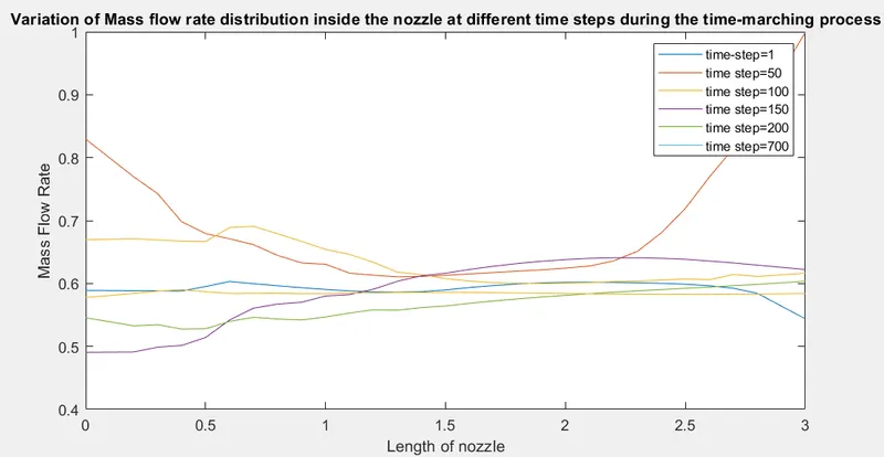
observation : there are fluctions in mass flow rate at lesser time steps because the solution hasnt converged yet ,

after 200 time step value mass flow rate becoming flat and the fluctuations tends to be reducing. after 700 time step value mass flow rate becomes straight , and this

satisfies Contuinity equation throghout the nozzle

2) Time wise Variations of primitive variables insie nozzle at throat section :

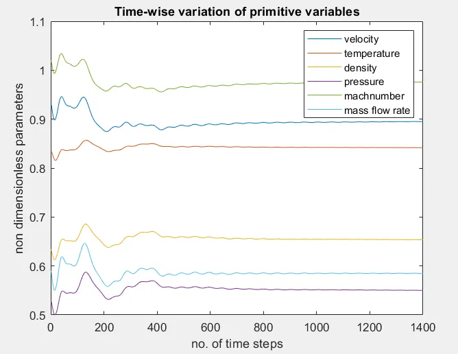
Observation :

we can see that there are fluctuations in values of primitive variables at intial stages at lesser time steps, this is also known as rubber band effect.

it takes some time marching to acheive orginial value of solution . values of primitive variables becoming straight line after 200 time steps.

3) Steady state distribution of primitive variables inside nozzle :

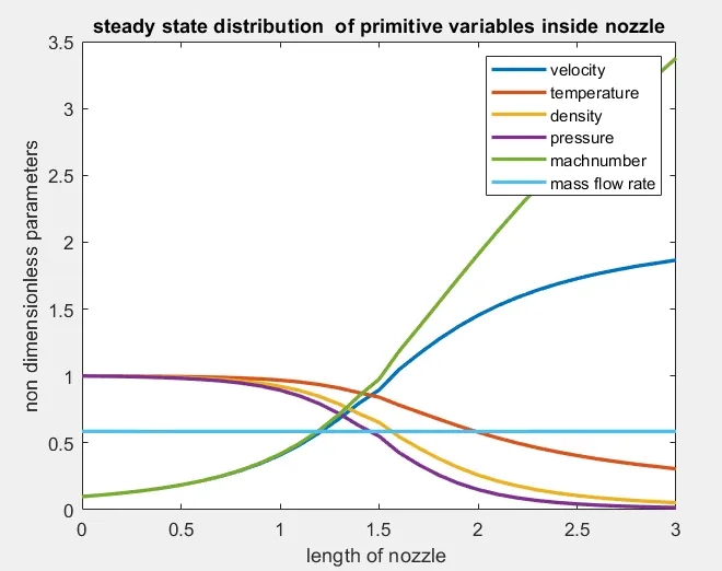
Observation : we can observe that Mach number and velocity increases with length of nozzle. pressure ,density and temperature decreases with increase in length of nozzle.

also we can observe here validation of contuinity equation , i.e. `(rhoVA)1 = (rhoVA)2` , because mass flow rate remaining constant throghout the length of nozzle

4) Variation of primitive variables with time steps :

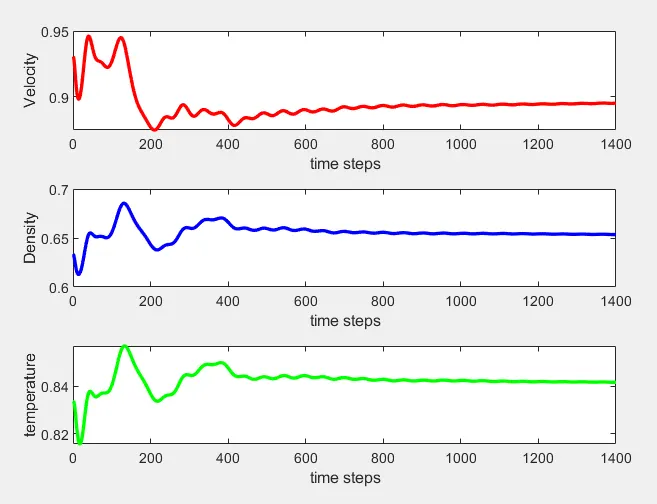
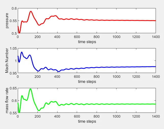
Observation : we can see from above plots variations of primitive variables with time steps, as they are first have more fluctuations and then

with time steps this fluctuation reduced.

Comparision of normalized mass flow rate distribution of both forms

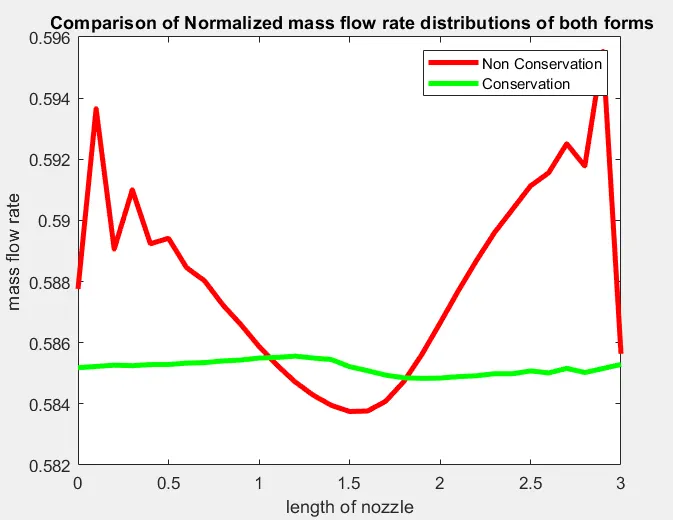
• Conservation form is good at preserving mass flow rate values throghout the domain because in conservation form mass flow rate is dependent variable
• we can see that Non conservation form have more variations at initially as well as at last , but in conservation form we get almost constant value of mass flow rate
• In non conservation form primitive variables are dpendent whether in conservation form mass flow rate is dependent
• steady state mass flow rate results are obtained from conservation form , which are much closer to analytical results which are `rho'*A'*V'`=0.579

Grid Independence test :

above we have calculated values of primitive variables for 31 grid points, but if we increase no. of grid points to 61

then whether the solution give same values of variables can be checked by performing grid independence test .

lets run this code for 61 grid points :

	`rho^star/(rho_0)`	`T^star/(T_0)`	`P^star/(P_0)`	Mach Number	Time(sec)
exact Analytical Solution	0.634	0.833	0.528	1
Non conservation form numerical results @ n=31	0.6387	0.8365	0.5342	0.9994	530.1108
conservation form numerical results @ n=31	0.6504	0.8400	0.5464	0.9817	415.6815
conservation form numerical results @ n=61	0.664	0.838	0.540	0.989	475.79

Observation :

• we can observe that Non conservation form have much more closer values to exact analytical values
• The accuracy of solution is increased after 61 grid points
• Hence our solution is grid independent

Conclusion :

1. Conservation form does good job of preserving values of mass flow rate, its produce better results for mass flow rate
2. Non conservation form yeild to smaller residuals and they decay to about `10^-1` after 1400 time steps , amount by which solution decays is also called as index of quality , hence Non conservation haave high index of quality when used in algorithm algorithm. Conservation form decays to only about `10^-6` after 1400 time steps , but this is okayto obtain steady state results
3. Non conservation form produces more accurate results for Primitive variables whether conservation form is good for producing results for flux variables
4. Solving the Conservation form requires much more efforts and accuracy in derivation as compared to non conservation form
5. Time required for Conservation form is less compared to Non conservation form , but this doesnt have much gap between both the time required.