Week 4.1 - Genetic Algorithm

Genetic Algorithm

Genetic Algorithms(GAs) are adaptive heuristic search algorithms that belong to the larger part of evolutionary algorithms. Genetic algorithms are based on the ideas of natural selection and genetics. These are intelligent exploitation of random search provided with historical data to direct the search into the region of better performance in solution space. They are commonly used to generate high-quality solutions for optimization problems and search problems.

Genetic algorithms simulate the process of natural selection which means those species who can adapt to changes in their environment are able to survive and reproduce and go to next generation. In simple words, they simulate “survival of the fittest” among individual of consecutive generation for solving a problem.

Foundation of Genetic Algorithms

Genetic algorithms are based on an analogy with genetic structure and behavior of chromosomes of the population. Following is the foundation of GAs based on this analogy –

1. Individual in population compete for resources and mate
2. Those individuals who are successful (fittest) then mate to create more offspring than others
3. Genes from “fittest” parent propagate throughout the generation, that is sometimes parents create offspring which is better than either parent.
4. Thus each successive generation is more suited for their environment

Matlab Code For Genetic Algorithm

close all 
clear all
clc
%% input parameters
x = linspace(0,0.6,150);
y = linspace(0,0.6,150);
num_cases = 50 
%% 2d meshgrid
[xx yy] = meshgrid(x,y);

%% stalagmatic function
for i = 1: length(xx);
    for j = 1: length(yy)
        input_vector(1) = xx(i,j);
        input_vector(2) = yy(i,j);
        f(i,j) = stalagmite(input_vector);
    end
end
figure(1);
surfc(x,y,f);
xlabel('X AXIS');
ylabel('Y AXIS');
zlabel('Z AXIS');
shading interp
[inputs, fval] = ga(@stalagmite,2);


%% stalagmite function
function [f] = stalagmite(input_vector);
           x = input_vector(1);
           y = input_vector(2);
           f1 = (sin(5.1*pi*x + 0.5)).^6;
           f2 = (sin(5.1*pi*y +0.5)).^6;
           f3 = exp(-4*log(2)*(x-0.0667).^2/0.64);
           f4 = exp(-4*log(2)*(y-0.0667).^2/0.64);
           f = (f1*f2*f3*f4);
           
end

syntax of ga

[inputs,fval] this give x and y values for which fval is minimum. if we run this code severel times using for loop we might get fval = 0

ga(@stalagmite,2) this shows us stalagmite function is solve for 2 variables

other forms of ga

x = ga(fun,nvars)
x = ga(fun,nvars,A,b)
x = ga(fun,nvars,A,b,Aeq,beq)
x = ga(fun,nvars,A,b,Aeq,beq,lb,ub)
x = ga(fun,nvars,A,b,Aeq,beq,lb,ub,nonlcon)
x = ga(fun,nvars,A,b,Aeq,beq,lb,ub,nonlcon,options)
x = ga(fun,nvars,A,b,[],[],lb,ub,nonlcon,IntCon)
x = ga(fun,nvars,A,b,[],[],lb,ub,nonlcon,IntCon,options)

fun = function

nvars = no of variables used

A = linear inequality constraints

b = linear inequality constraints

Aeq = linear inequality constraints

beq = linear inequality constraints

lb = Lower bound on x

ub = upper bound on x

nonlcon = Nonlinear constraint function

IntCon = Indices of integer variables

options = Options created using optimoptions or an options structure

Plot i got from this code

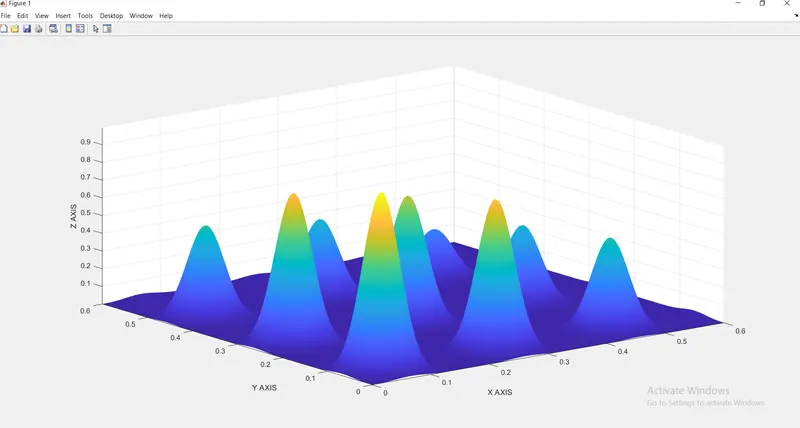
this results shows us global minima for one given iterations for accurately predicting global maxima we need to increase no. of iterations.

if we ran this function for severel iterations it will give us same optimized maxima every time. three stuies are made while performing this process as follows

1 unbounded inputs -

2 bounded inputs -restricting limits

3 by increasing no of iterations

For finding global maxima

when we run code by imposing negetive sign in equation we get global maxima

Full program

close all 
clear all
clc
%% input parameters
x = linspace(0,0.6,150);
y = linspace(0,0.6,150);
num_cases = 50 
%% 2d meshgrid
[xx yy] = meshgrid(x,y);

%% stalagmatic function
for i = 1: length(xx);
    for j = 1: length(yy)
        input_vector(1) = xx(i,j);
        input_vector(2) = yy(i,j);
        f(i,j) = stalagmite(input_vector);
    end
end
figure(1);
surfc(x,y,f);
xlabel('X AXIS');
ylabel('Y AXIS');
zlabel('Z AXIS');
shading interp
[inputs, fval] = ga(@stalagmite,2);




%% study1 : statistical behaviour 
tic
for i = 1 : num_cases
    [inputs,fopt(i)] =ga(@stalagmite,2);
    xopt(i)    = inputs(1); % for storing x value from inputs result 
    yopt (i)      = inputs(2); % for storing y value from inputs result 
  
end

study1_time = toc; % timer for study 
figure(2);
subplot(2,1,1); % subplot command shows that we divided grid into 2x1 matrix and using 1st part for plotting 
hold on
surfc(x,y,f)
shading interp % shading interp used for removing unneccesery lines on graph 
plot3(xopt,yopt,fopt,'marker','o','markersize',5,'markerfacecolor','r');
title('unbounded inputs');
subplot(2,1,2); % subplot command shows that we divided grid into 2x1 matrix and using 1st part for plotting 
plot(fopt);
xlabel('Iterations');
ylabel('function minimum');

%% Study 2 - statistical behaviour with upper an lower bounds 
tic
for i = 1 : num_cases
    [inputs,fopt(i)] =ga(@stalagmite,2,[],[],[],[],[0;0],[1;]);
    xopt(i)    = inputs(1); % for storing x value from inputs result 
    yopt (i)      = inputs(2); % for storing y value from inputs result 
  
end
study2_time = toc
figure(3);
subplot(2,1,1); % subplot command shows that we divided grid into 2x1 matrix and using 1st part for plotting 
hold on
surfc(x,y,f)
shading interp % shading interp used for removing unneccesery lines on graph 
plot3(xopt,yopt,fopt,'marker','o','markersize',5,'markerfacecolor','r');
title('bounded inputs');
subplot(2,1,2); % subplot command shows that we divided grid into 2x1 matrix and using 1st part for plotting 
plot(fopt);
xlabel('Iterations');
ylabel('function minimum');

%% study3 - increasing GA iterations 
options = optimoptions('ga');
options = optimoptions(options,'populationsize',170)

tic

for i = 1 : num_cases
    [inputs,fopt(i)] =ga(@stalagmite,2,[],[],[],[],[0;0],[1;],[],[]);
    xopt(i)    = inputs(1); % for storing x value from inputs result 
    yopt (i)      = inputs(2); % for storing y value from inputs result 
  
end
study3_time = toc
figure(4);
subplot(2,1,1); % subplot command shows that we divided grid into 2x1 matrix and using 1st part for plotting 
hold on
surfc(x,y,f)
shading interp % shading interp used for removing unneccesery lines on graph 
plot3(xopt,yopt,fopt,'marker','o','markersize',5,'markerfacecolor','r');
title('bounded inputs');
subplot(2,1,2); % subplot command shows that we divided grid into 2x1 matrix and using 1st part for plotting 
plot(fopt);
xlabel('Iterations');
ylabel('function minimum');

Results:

Study 1

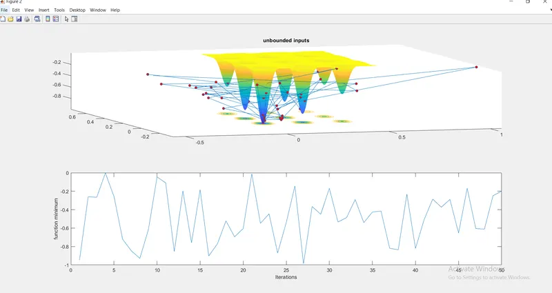
study 1 time = 4.4445 sec

Study 2

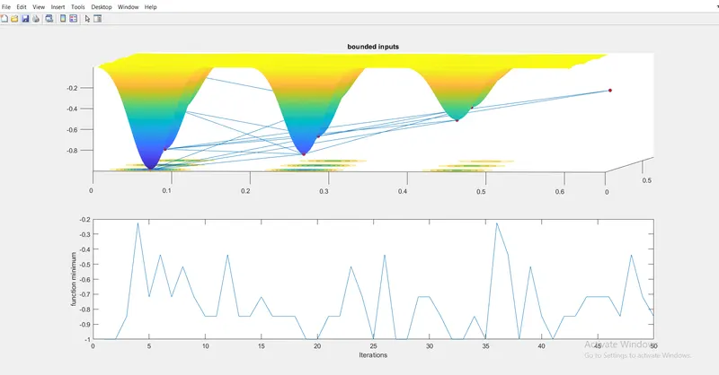
study2 time = 5.8438 sec

Study 3

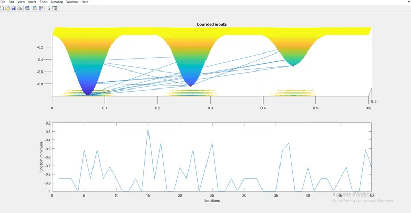
study3 time = 5.9208 sec

Conclusion:

i got global maxima = 1