Week 3 - Solving second order ODEs

https://youtu.be/JyE8Jn_Obbwhttps://youtu.be/JyE8Jn_Obbw

clear all 
close all 
clc

%% input parameters ;
b = 0.05; % b= damping coefficient;
g = 9.81 ; % gravitational constant(m/s^2); 
l = 1; %length (m);
m = 1; % mass(kg)
t_span = linspace(0,20,500);
%% initial conditions
theta_0 = [0;3];
% where angular displacement(theta) = 0, angular velocity(dtheta/dt) = 3 rad/s . we need to specify this
% condition because ode45 function will require some initial condition for
% solution.

%% solving differential equation using ode45.
[t,results] = ode45(@(t,theta)damfunc(t,theta,b,g,l,m),t_span,theta_0);
% here results show us theta and dtheta/dt in 500*2 form .
%% plotting
figure(1)
plot(t,results(:,1));
hold on;
plot(t,results(:,2));
ylabel('VARIABLES');
xlabel('TIME');
% legend command is used to represent curves
legend('angular dispacement','angular velocity');
figure(2)
ct = 1 
for i =1:length(results(:,1)); % For loop is performed by taking length of angular dispacement. 
    x0 = 0
    y0 = 0
    x1 = l*sin(results(i,1));
    y1 = -l*cos(results(i,1));
    plot([1 1], [0 0 ], 'linewidth',4,'color','g');
    hold on
    % line  for pendulam 
    line([ x0 x1],[y0 y1],'linewidth',2,'color','b');
    hold on 
    % fixed support 
   line([-1 1],[0 0],'color','k','linewidth',6);
   hold on
    % bob by marker command 
    plot(x1,y1,'-o','markers',20,'markerfacecolor','r')
    grid on
    axis([-1.5 1.5 -1.5 0.5])
    pause(0.003)
    hold off
    M(ct) = getframe(gcf)
    ct = ct+1
end
movie(M)
videofile = VideoWriter('Pendulum_motion.avi','uncompressed avi');
open(videofile)
writeVideo(videofile,M)
close(videofile)

RESULTS :

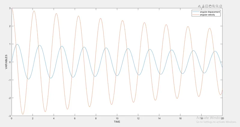
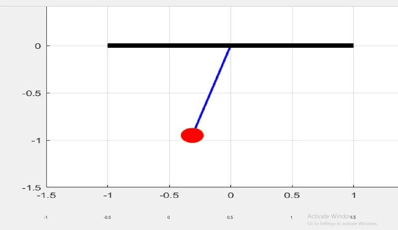
we can see that code works perfectly fine and we got plot for damping angular velocity and displacement.

%% Function which i have used saved by damfunc.m

function [dtheta_dt] = damfunc(t,theta,b,g,l,m);

theta1= theta(1)
theta2 = theta(2);
dtheta1_dt = theta2;
dtheta2_dt = -(b/m)*theta2-(g/l)*sin(theta1);
dtheta_dt = [dtheta1_dt;dtheta2_dt]
end