Simulation of a 1D Super-sonic nozzle flow simulation using Macormack Method
Introduction:
Isentropic Process:
A process during which entropy remains constant is called an isentropic process.Change in entropy araises due to heat transfer and irreversiblities.
Isentropic process used in thermodynamics to imply an internally reversible,adiabatic process
Adiabatic Process:
A Process during which there is no heat transfer is called an adiabatic process.
Reversible process:
A reversible process is defined as a process that can be reversed without leaving any traces on the surroundings.That is,both the system and the surroundings returned to their initial states.
Isentropic Flow:
Isentropic flow occurs when the change in flow variables is small and gradual .
The generation of sound waves in an isentropic flow
Subsonic-Supersonic nozzle:
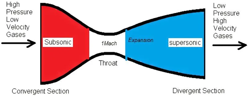
convergent-divergent nozzle is a tube which is pinched in the middle, making a carefully balanced, asymmetric hourglass shape. It is used to accelerate a compressible fluid to supersonic speeds in the axial (thrust) direction, by converting the thermal energy of the flow into kinetic energy. convergent-divergent nozzles are widely used in some types of steam turbines and rocket engine nozzles. It also sees use in supersonic jet engines.
Reason for choosing a 1D or 2D or 3D:
A flow field is best characterised by the velocity distribution.if flow velocity varies on the physical three dimensional geometry on all three directions then need to render a 3D dimensional analysis.if flow velocity varies of two or one directions on the three dimensional geometry then need to render two or one dimensional analysis.in a real world ignoring a small variation to render a two or one dimensional analysis.
Quasi equilibrium process:
It can be viewed as sufficiently slow process to adjust itself internally,so that properties in one part of the system donot change faster than those at the other parts of the system.
Derivation:
Reynolds Transport Theorem:
This theorem is used to convert the governing equations of the system to the Control Volume.In fluids a system approach is complicated due to tracking of each and every particle where control volume approach is a region choosen for study it is bit easy mathematically to solve a problems
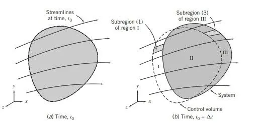
Consider a system and control at time t where both are at same location, at time `t+delt` control volume is fixed ,where it is located at the same place at the time t,system changes a location from time at t.
system indicated as grey colour in the figure.
B represents extensive property
b represents intensive property
At time t
`underset(sys,t)(B)=underset(CV,t)(B)`
At time `t+delt`
`underset(sys,t+delt)(B)=underset(CV,t+delt)(B)-underset(I,t+delt)(B)+underset(III,t+delt)(B)`
Changes in system property with respect to the time
`frac{underset(sys,t+delt)(B)-underset(sys,t)(B)}{delt}=frac{underset(CV,t+delt)(B)-underset(CV,t)(B)}{delt}-frac{underset(I,t+delt)(B)}{delt}+frac{underset(III,t+delt)(B)}{delt}`
at `delt rarr0`
`frac{underset(III,t+delt)(B)}{delt}=underset(3)(b)*underset(3)(rho)*underset(3)(v)*underset(3)(delt)*underset(3)(A)`
`frac{underset(I,t+delt)(B)}{delt}=underset(1)(b)*underset(1)(rho)*underset(1)(v)*underset(1)(delt)*underset(1)(A)`
`underset(n)(rarr)`indicates a direction vector is a outward normal,velocity and direction vector in the same direction in the positive sign and vice versa
`frac{underset(III,t+delt)(B)}{delt}-frac{underset(I,t+delt)(B)}{delt}=intb*rho*v.overset(rarr)(n)*delA`
R.H.S 1st term consists of control volume integral and 2nd term consists of control surface integral
`frac{underset(sys)(delB)}{delt}=frac{d}{dt}intpbdV+intb*rho*v.overset(rarr)(n)*delA`
Flow field variables in Non dimensional form
`T'=frac{T}{underset(o)(T)}`
`rho'=frac{rho}{underset(o)(rho)}`
`x'=frac{x}{L}`
`v'=v/underset(o)(a)`
`underset(o)(a)=sqrt( gamma *R*underset(o)(T))`
`t'=frac{t}{frac{L}{underset(o)(a)}`
`A'=frac{A}{overset(*)(A)}`
`p=gamma*R*T`
1.Continuity equation
Conservation of mass means change in mass is zero or constant.
`0=int intintfrac{delrho}{delt}*dV+int int rho.v.underset(n)(rarr)*dA`
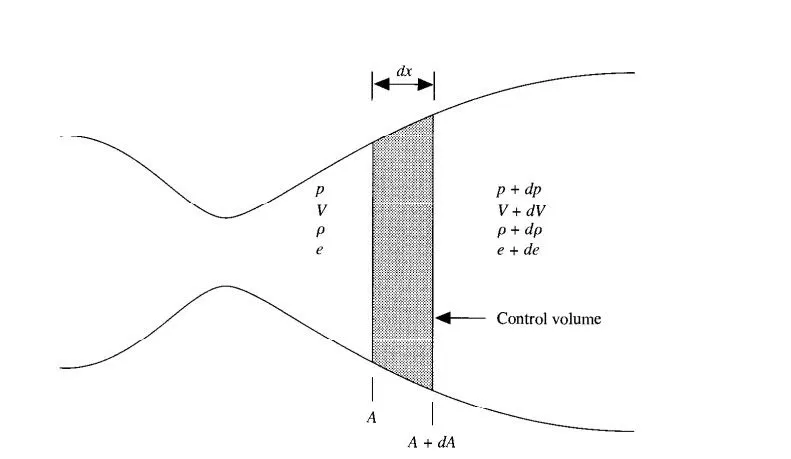
-negative sign is due to velocity and outward normal vector is in oppposite direction.
`int int rho*v*dA=-rho*v*a+(rho+drho)*(v+dv)*(A+dA)`
`intint(p.dA)=-pA+(p+dp)(A+dA)-2p(frac{dA}{2})`
Expanding and neglecting the product of differentials
`int int rho*v*dA=drho*v*A+ rho*dv*A+rho*v*dA`
`int int rho*v*dA=d(rho*v*A)`
where area is uniform at the cross section
`frac{del}{del t}intintintrho*dV=frac{del }{del t}(rho*A*dx)`
dividing by dx
`frac{del}{del t}(rho*A)+frac{del}{del x}(rho*v*A)=0`
above equation is conservative form.
Applying a nondimensional flow variable relation to the conservation form
`frac{underset(0)(a)*underset(0)(rho)*underset(*)(A)}{L}[frac{del(rho'A')}{delt'}+frac{del(rho'A'v')}{delx'}]=0`
`frac{del(rho'A')}{delt'}+frac{del(rho'A'v')}{delx'}=0` conservation form of continuity equation
Applying a nondimensional flow variable relation to the non-conservation form
`frac{del}{del t}(rho*A)+v*A*frac{delrho}{del x}+rho*v*frac{del A}{del x}+rho*A*frac{del v}{del x}=0`
area is not a dependent on t
`frac{del rho'}{del t}=-v'frac{del rho'}{del x'}-rho'v'frac{del ln A'}{del x'}-rho'frac{delv'}{delx'}`non-conservation form of continuity equation
2.Momentum Equation:
`-intint(P.dA)=frac{del }{del t}int intintrho *v*dV+int int rho*v*v*dA`
where Area is uniform over a cross section
`frac{del}{del t}int intintrho *v*dV=frac{del }{del t}intrho*v*A*dx`
`intintrho*v*v*dA=-rho*v^2*A+(rho + drho)(v+dv)^2(A+dA)`
`intintrho *v*v*dA=d(rho*v^2*A)`
`intint(p.dA)=-pA+(p+dp)(A+dA)-2p*frac{dA}{2}`
`-Adp=d(rho*v^2*A)+frac{del}{del t}(rho*v*A*dx)`
Dividing By dx
`frac{del}{del t}(rho*v*A)+frac{del }{del x}(rho*v^2*A)=-Afrac{del p}{dx}`
Above equation is a conservative form
Continuity equation multiply with Velocity
`v*frac{del}{delt} (rho*A)+v*frac{del}{delx}(rho*v*A)=0`
subtract Momentum conservation equation with above equation
`frac{del}{delt}(rho*v*A)-v*frac{del}{delt}(rho*A)+frac{del}{delx}(rho*v^2*A)-v*frac{del}{delx}(rho*v*A)=-Afrac{dp}{dx}`
dividing by A
`rho*frac{delv}{delt}+rho*vfrac{delv}{delx}=-frac{dp}{dx}`
Above equation is a non-conservative form.
To eliminate pressure term
`p=rho*R*T`
differentiating the above equation
`frac{del p}{del x}=R[T*frac{del rho}{delx}+rho*frac{del T}{del x}]`
Applying pressure term expansion on the non-conservation form of equation
`rho frac{delv}{delt}+rho*vfrac{delv}{delx}=-R[T*frac{del rho}{delx}+rho*frac{del T}{del x}]`
Applying non-dimensional variables in conservative form
`frac{del}{del t}(rho*v*A)+frac{del}{del x}(rho*v^2*A)=-Afrac{dp}{dx}`
`frac{underset(o)(rho)*underset(o)(a^2)overset(*)(A)}{L}[frac{del(rho'*v'*A')}{delt'}]+frac{underset(o)(rho)*underset(o)(a^2)overset(*)(A)}{L}[frac{del(rho'*v'^2*A')}{delx'}]=[frac{overset(*)(A)*A'*underset(o)(rho)*R*underset(o)(T)}{L}]*frac{delp'}{delx'}`
After cancelling and chain rule expansion for the RHS
`frac{del(rho'v'A')}{delt'}+frac{del((rho'v'^2A')+frac{1}{gamma}*p'A')}{delx'}=frac{1}{gamma}p'frac{delA'}{delx'}` conservation form of momentum equation
Applying non-dimensional variables in non conservative form
`rho frac{delv}{delt}+rho*vfrac{delv}{delx}=-R[T*frac{del rho}{delx}+rho*frac{del T}{del x}]`
dividing by `rho'`
`frac{delv'}{delt'}=-v'frac{del v'}{del x'}-frac{1}{gamma}[frac{T'}{rho'}frac{del rho'}{del x'}+frac{delT'}{delx'}]` non-consevation form of momentum equation
3.Energy Equation:
`frac{del}{delt}int int int rho*(e+frac{v^2}{2})dV+intint rho*(e+frac{v^2}{2})*v*dA=-int int (pv dA)`
After substituting for uniform area cross section and integrating we will get
`frac{del}{delt}[ rho*(e+frac{v^2}{2})*A*dx]+d[ rho*(e+frac{v^2}{2})*v*A]=-d(pvA)`
Dividing by dx
`frac{del[ rho*(e+frac{v^2}{2})*A]}{delt}+frac{del[ rho*(e+frac{v^2}{2})*v*A]}{del x}=-frac{del(pvA)}{del x}`
Above equation is a conservation form of energy equation
spiltting the energy term
`frac{del[ rho*e*A]}{delt}+frac{del[ rho*e*v*A]}{del x}=-p*frac{del(vA)}{del x}`
To obtain the non conversation form, multiply e with continuity equation
`e*frac{del}{del t}(rho*A)+e*frac{del}{del x}(rho*v*A)=0`
Above equation subtracting with splitted energy term
`rho * A frac{del e}{del t}+rho *A*v frac{del e}{del x}=-pfrac{del(Av)}{delx}`
Diving A on the above equation
`rho *frac{del e}{del t}+rho*v*frac{del e}{delx}=-pfrac{delv}{del x}-pvfrac{del( ln A)}{delx}`
Above equation is a non-conservation form of energy equation
`e=underset(v)(C)*T`
Substitute energy formula in the non conservation form of energy equation
`rho*underset(v)(C) *frac{del T}{del t}+rho*underset(v)(C)* v*frac{del T}{delx}=-pfrac{delv}{del x}-pvfrac{del( ln A)}{delx}`
To eliminate pressure term
`p=rho*R*T`
differentiating the above equation
`frac{delp}{del x}=R*[T*frac{del rho}{delx}+rho*frac{delT}{delx}]`
Applying pressure formula on non conservation form of energy equation
`rho*underset(v)(C) *frac{del T}{del t}+rho*underset(v)(C)* v*frac{del T}{delx}=-rho*R*T[frac{delv}{del x}+vfrac{del( ln A)}{delx}]`
Applying non-dimensional variables in conservative form
`frac{del(rho'A'(frac{e}{gamma-1}+frac{gammav'^2}{2}))){delt'}+frac{del(rho'v'A'(frac{e}{gamma-1}+frac{gamma*v'^2}{2})+p'v'A')}{del x'}=0` conservation form of energy equation
Applying non-dimensional variables in non-conservative form
dividing by `rho'`
`frac{del T'}{delt}=-v'frac{del T'}{delx'}-T'(gamma-1)[frac{delv'}{delx'}+v'frac{del lnA'}{delx'}]` non-conservation form of energy equation
Maccormacks method:
Like lax-wendroff method,it is also the second order explicit finite difference method in both space and time.It is easiest to understand and program ,these are the advantages over the lax wendroff technique
Maccormacks technique is a predictor-corrector Technique
Predictor step is carried out by forward differencing Explicit method.
`frac{delv'}{delt'}=-v'frac{del v'}{del x'}-frac{1}{gamma}[frac{T'}{rho'}frac{del rho'}{del x'}+frac{delT'}{delx'}]`
`underset(i)((frac{delv'}{delt'})^t)=v'^tfrac{(underset(i+1)(v')^t-underset(i)(v')^t)}{trianglex}-frac{1}{gamma}(frac{underset(i+1)(T')^t-underset(i)(T')^t}{trianglex}+frac{underset(i)(T')^t}{underset(i)(rho')^t}frac{underset(i+1)(rho')^t-underset(i)(rho')^t}{trianglex})`
Solution Update
`underset(i)(v'^(-t+dt))=underset(i)(v'^t)+underset(i)((frac{delv'}{delt'})^t)*delt'`
Corrector step is carried out by rearward differences
`(underset(i)(frac{del v'}{delt'}))^(-t+del t)=(underset(i)(v'))^(-t'+delt')frac{(underset(i)(v'))^(-t'+delt')-(underset(i-1)(v'))^(-t'+delt')}{delx'}-frac{1}{gamma}(frac{underset(i-1)(T')^(-t'+delt')-underset(i)(T')^(-t'+delt')}{del x'}+frac{underset(i)(T')^(-t'+delt')}{underset(i)(rho')^(-t'+delt')}frac{underset(i-1)(rho')^(-t'+delt')-underset(i)(rho')^(-t'+delt')}{del x'})`
Average time derivatives
`(underset(av)(frac{del v'}{del t'}))=frac{1}{2}((underset(i)(frac{delv'}{delt'})^t)+(underset(i)(frac{delv'}{delt'})^(t'+delt')))`
Solution update
`underset(i)(v'^(t'+del t'))=underset(i)(v'^(t'))+underset(av)((frac{delv'}{delt'}))*delt'`
In a similar way ,maccormack method will be implemented for non-conservative form of continuity and energy equation
Conservative form rearranged as
`underset(1)(U)=rho'A'`
`underset(1)(F)=rho'A'v'`
`frac{del underset(1)(U)}{del t'}=-frac{del underset(1)(F)}{delx'}` Continuity Equation
`underset(2)(U)=rho'A'v'`
`underset(2)(F)=rho'A'v'^2+frac{1}{gamma}p'A'`
`underset(2)(J)=frac{1}{gamma}p'frac{del A'}{del x'}`
`frac{del underset(2)(U)}{del t'}=-frac{del underset(2)(F)}{delx'}+underset(2)(J)` Momentum Equation
`underset(3)(U)=rho'(frac{e'}{gamma-1}+frac{gamma}{2}v'^2)A'`
`underset(3)(F)=rho'(frac{e'}{gamma-1}+frac{gamma}{2}v'^2)v'A'+p'A'v'`
`frac{del underset(3)(U)}{del t'}=-frac{del underset(3)(F)}{del x'}` Energy Equation
Initial conditions and Boundary conditions
i.conservation form
%initial condition
for `0<=x'<=0.5`
`rho'=1`
`T'=1`
for `0.5<=x'<=1.5`
`rho'=1.0-0.366*(x'-0.5)`
`T'=1.0-0.167(x'-0.5)`
for `1.5<=x'<=3.5`
`rho'=0.634-0.3879*(x'-1.5)`
`T'=0.833-0.3507*(x'-1.5)`
U2=0.59
`A=1+2.2*(x'-1.5)^2`
%Boundary conditions
inlet
`U1(1)=A'`
`U2(1)=2*U2(2)-U2(3)`
`U3(1)=U1(1)(frac{T'}{gamma-1}+frac{gamma}{2}*V'^2)`
outlet
`U1(N)=2*U1(N-1)-U1(N-2)`
`U2(N)=2*U2(N-1)-U2(N-2)`
`U3(N)=2*U3(N-1)-U3(N-2)`
ii.Non-conservative form
%initial conditions
`rho'=1-0.3146*x'`
`T'=1-0.2314*x'`
`V'=(0.1+1.09*x')*T^(1/2)`
`A=1+2.2*(x'-1.5)^2`
%boundary conditions
inlet
`T'(1)=1`
`rho'(1)=1`
`V'(1)=2*V'(2)-V'(3)`
outlet
`V'(N)=2*V'(N-1)-V'(N-2)`
`rho'(N)=2*rho'(N-1)-rho'(N-2)`
`T'(N)=2*T'(N-1)-T'(N-2)`
TimeStep
`dt=frac{C*dx}{v+a}`
a-speed of sound
v-velocity of flow
c-courant number
At each grid point is calculated.due to unsteady problem have to select the minimum time step
PROGRAM:
Main program
clc
clear all
close all
nt=1400;
n=31
x=linspace(0,3,n);
gamma=1.4
A=1+(2.2*((x-1.5).^2));
C=0.5
%% Analytical
rho_stag=1;
Temp_Stag=1;
m=0;
b=A*-1
tic
for i=1:1:n
    residual=1;
    while residual > 1e-9
        m=m+1e-4
        residual =((1/(m^2))*((2/(gamma+1))*(1+((gamma-1)/2)*(m^2)))^((gamma+1)/(gamma-1)))-A(i)^2
        if i>=17 && i<=31
           residual=residual*-1;
        end
    end
    mach_no(i)=m;
end


temp_an=(1+((gamma-1)/2).*mach_no.^2).^-1;
density_an=(1+((gamma-1)/2).*mach_no.^2).^(-1/(gamma-1));
Pressure_an=density_an.*temp_an;
velocity_an=mach_no.*sqrt(temp_an)
Time_an=toc
%% non-conservation
tic
[rho_nc,T_nc,v_nc,mfw,density_non_con,Temp_non_con,velocity_non_con,k,drho_dt_avg,dT_dt_avg,dv_dt_avg,Pressure_non_con,time_step_non_con,p_nc,Mach_number,non_con_mass_flow_rate,non_con_time_ratio]=non_conservation_form(x,A,n,gamma,nt,C)
non_Con_execution_time=toc
%figure(1)
%plot(x,density_an,x,density_non_con);
%legend('Analytical','non-conservation');
figure(2)
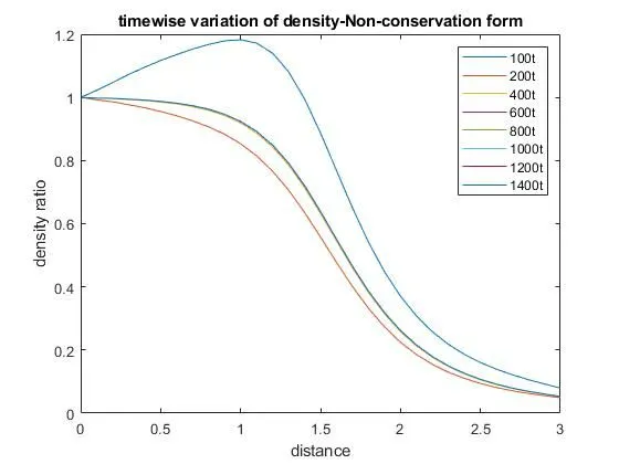
plot(x,rho_nc(1,:),x,rho_nc(2,:),x,rho_nc(3,:),x,rho_nc(4,:),x,rho_nc(5,:),x,rho_nc(6,:),x,rho_nc(7,:),x,rho_nc(8,:))
xlabel('distance')
ylabel('density ratio')
title('timewise variation of density-Non-conservation form')
legend('100t','200t','400t','600t','800t','1000t','1200t','1400t')
figure(3)
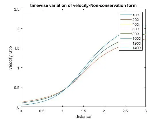
plot(x,v_nc(1,:),x,v_nc(2,:),x,v_nc(3,:),x,v_nc(4,:),x,v_nc(5,:),x,v_nc(6,:),x,v_nc(7,:),x,v_nc(8,:))
legend('100t','200t','400t','600t','800t','1000t','1200t','1400t')
xlabel('distance')
ylabel('velocity ratio')
title('timewise variation of velocity-Non-conservation form')
figure(4)
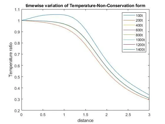
plot(x,T_nc(1,:),x,T_nc(2,:),x,T_nc(3,:),x,T_nc(4,:),x,T_nc(5,:),x,T_nc(6,:),x,T_nc(7,:),x,T_nc(8,:))
legend('100t','200t','400t','600t','800t','1000t','1200t','1400t')
xlabel('distance')
ylabel('Temperature ratio')
title('timewise variation of Temperature-Non-Conservation form')
figure(5)
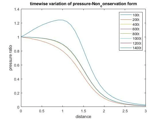
plot(x,p_nc(1,:),x,p_nc(2,:),x,p_nc(3,:),x,p_nc(4,:),x,p_nc(5,:),x,p_nc(6,:),x,p_nc(7,:),x,p_nc(8,:))
legend('100t','200t','400t','600t','800t','1000t','1200t','1400t')
xlabel('distance')
ylabel('pressure ratio')
title('timewise variation of pressure-Non_conservation form')
figure(6)
plot(x,mfw(1,:),x,mfw(2,:),x,mfw(3,:),x,mfw(4,:),x,mfw(5,:),x,mfw(6,:),x,mfw(7,:),x,mfw(8,:))
legend('100t','200t','400t','600t','800t','1000t','1200t','1400t')
xlabel('distance')
ylabel('mass flow rate')
title('timewise variation of mass flow rate-Non-conservation form')


%% conservation
tic
[rho_c,T_c,v_c,mfw_c,density_con,Temp_con,velocity_con,U1,U2,U3,Pressure_con,Mach_no_con,p_c,Con_mass_flow_rate,con_time_ratio]=conservative_form(x,A,n,gamma,nt,C)
Con_execution_time=toc
figure(7)
plot(x,rho_c(1,:),x,rho_c(2,:),x,rho_c(3,:),x,rho_c(4,:),x,rho_c(5,:),x,rho_c(6,:),x,rho_c(7,:),x,rho_c(8,:))
xlabel('distance')
ylabel('density ratio')
title('timewise variation of density-Conservation form')
legend('100t','200t','400t','600t','800t','1000t','1200t','1400t')
figure(8)
plot(x,v_c(1,:),x,v_c(2,:),x,v_c(3,:),x,v_c(4,:),x,v_c(5,:),x,v_c(6,:),x,v_c(7,:),x,v_c(8,:))
legend('100t','200t','400t','600t','800t','1000t','1200t','1400t')
xlabel('distance')
ylabel('velocity ratio')
title('timewise variation of velocity-Conservation form')
figure(9)
plot(x,T_c(1,:),x,T_c(2,:),x,T_c(3,:),x,T_c(4,:),x,T_c(5,:),x,T_c(6,:),x,T_c(7,:),x,T_c(8,:))
legend('100t','200t','400t','600t','800t','1000t','1200t','1400t')
xlabel('distance')
ylabel('Temperature ratio')
title('timewise variation of Temperature-Conservation form')
figure(10)
plot(x,p_c(1,:),x,p_c(2,:),x,p_c(3,:),x,p_c(4,:),x,p_c(5,:),x,p_c(6,:),x,p_c(7,:),x,p_c(8,:))
legend('100t','200t','400t','600t','800t','1000t','1200t','1400t')
xlabel('distance')
ylabel('pressure ratio')
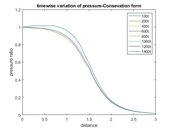
title('timewise variation of pressure-Consevation form')
figure(11)
plot(x,mfw_c(1,:),x,mfw_c(2,:),x,mfw_c(3,:),x,mfw_c(4,:),x,mfw_c(5,:),x,mfw_c(6,:),x,mfw_c(7,:),x,mfw_c(8,:))
legend('100t','200t','400t','600t','800t','1000t','1200t','1400t')
xlabel('distance')
ylabel('mass flow rate')
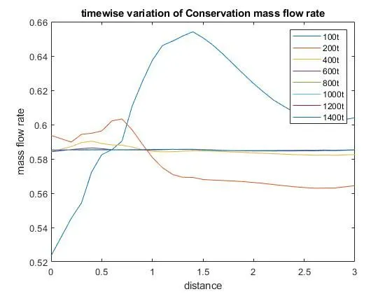
title('timewise variation of Conservation mass flow rate')
%% Comparision plots
figure(1)
subplot(3,1,1)
plot(x,density_an,'-.',x,density_non_con,'r',x,density_con,'*');
hold on
plot([x(1) x(16) x(16)],[density_an(16) density_an(16) 0],'--','color','b')
xticks(1.5)
yticks(density_an(16))
yticklabels(density_an(16))
xlabel('non-dimesional distance')
ylabel('Density ratio')
axis([0 3 0 1.5]);
legend('Analytical','non-conservation form','conversation form');
hold off
subplot(3,1,2)
plot(x,temp_an,'-.',x,Temp_non_con,'r',x,Temp_con,'*');
hold on
plot([x(1) x(16) x(16)],[temp_an(16) temp_an(16) 0],'--','color','b')
xticks(1.5)
yticks(temp_an(16))
yticklabels(temp_an(16))
xlabel('non-dimesional distance')
ylabel('Temperature ratio')
axis([0 3 0 1.5]);
legend('Analytical','non-conservation form','conversation form');
hold off
subplot(3,1,3)
plot(x,Pressure_an,'-.',x,Pressure_non_con,'r',x,Pressure_con,'*');
hold on
plot([x(1) x(16) x(16)],[Pressure_an(16) Pressure_an(16) 0],'--','color','b')
xticks(1.5)
yticks(Pressure_an(16))
yticklabels(Pressure_an(16))
xlabel('non-dimesional distance')
ylabel('Pressure ratio')
axis([0 3 0 1.5]);
legend('Analytical','non-conservation form','conversation form');
hold off
figure(12)
subplot(2,1,1)
plot(x,mach_no,'-.',x,Mach_number,'r',x,Mach_no_con,'*');
hold on
plot([x(1) x(16) x(16)],[mach_no(16) mach_no(16) 0],'--','color','b')
xticks(1.5)
yticks(mach_no(16))
yticklabels(mach_no(16))
xlabel('non-dimesional distance')
ylabel('Mach number')
axis([0 3 0 4]);
legend('Analytical','non-conservation form','Conservation form');
hold off
subplot(2,1,2)
plot(x,velocity_non_con,'r',x,velocity_con,'*');
hold on
plot([x(1) x(16) x(16)],[velocity_non_con(16) velocity_non_con(16) 0],'--','color','b')
xticks(1.5)
yticks(velocity_non_con(16))
yticklabels(velocity_non_con(16))
xlabel('non-dimesional distance')
ylabel('Velocity ratio')
axis([0 3 0 4]);
legend('non-conservative form','Conservative form');
hold off
figure(13)
plot(x,Con_mass_flow_rate,'r',x,non_con_mass_flow_rate,'g');
xlabel('non-dimesional distance')
ylabel('Mass flow rate')
legend('conservative form','non-Conservative form');
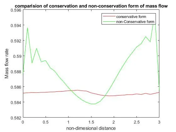
title('comparision of conservation and non-conservation form of mass flow')
%% Grid independence
x=linspace(0,3,61)
A=1+(2.2*((x-1.5).^2));
tic
[rho_nc_61,T_nc_61,v_nc_61,mfw_61,density_non_con_61,Temp_non_con_61,velocity_non_con_61,k,drho_dt_avg,dT_dt_avg,dv_dt_avg,Pressure_non_con_61,time_step_non_con,p_nc_61,Mach_number_61,non_con_mass_flow_rate_61,non_con_time_ratio_61]=non_conservation_form(x,A,61,gamma,nt,C)
non_con_execution_time_61=toc
tic
[rho_c_61,T_c_61,v_c_61,mfw_c_61,density_con_61,Temp_con_61,velocity_con_61,U1_61,U2_61,U3_61,Pressure_con_61,Mach_no_con_61,p_c_61,Con_mass_flow_rate_61,con_time_ratio_61]=conservative_form(x,A,61,gamma,nt,C)
con_execution_time_61=toc
filename='gridindependence.xlsx'
a="density ratio"
b="61 Grid Points"
c="conservation form"
d="non-conservation form"
e="31 Grid Points"
Density_ratio_No_of_grid_points=[b;b;e;e;e]
Density_ratio_Numerical_solution_form=[c;d;c;d;"Analytical_form"]
Density_ratio_values_at_throat=[density_con_61(31);density_non_con_61(31);density_con(16);density_con(16);density_an(16)]
Execution_time=[con_execution_time_61;non_con_execution_time_61;Con_execution_time;non_Con_execution_time;Time_an];
Nondimensional_time=[con_time_ratio_61;non_con_time_ratio_61;con_time_ratio;non_con_time_ratio;0];
W=table(Density_ratio_No_of_grid_points,Density_ratio_Numerical_solution_form,Density_ratio_values_at_throat,Execution_time,Nondimensional_time)
writetable(W,'Gridindependence.xls','Sheet',1,'Range','A1:E6')

Velocity_ratio_No_of_grid_points=[b;b;e;e;e]
Velocity_ratio_Numerical_solution_form=[c;d;c;d;"Analytical_Form"]
Velocity_ratio_values_at_throat=[velocity_con_61(31);velocity_non_con_61(31);velocity_con(16);velocity_non_con(16);velocity_an(16)]
W=table(Velocity_ratio_No_of_grid_points,Velocity_ratio_Numerical_solution_form,Velocity_ratio_values_at_throat)
writetable(W,'Gridindependence.xls','Sheet',1,'Range','A8:C13')

Temperature_ratio_No_of_grid_points=[b;b;e;e;e]
Temperature_ratio_Numerical_solution_form=[c;d;c;d;"Analytical_Form"]
Temperature_ratio_values_at_throat=[Temp_con_61(31);Temp_non_con_61(31);Temp_con(16);Temp_non_con(16);temp_an(16)]
W=table(Temperature_ratio_No_of_grid_points,Temperature_ratio_Numerical_solution_form,Temperature_ratio_values_at_throat)
writetable(W,'Gridindependence.xls','Sheet',1,'Range','A15:C20')

Pressure_ratio_No_of_grid_points=[b;b;e;e;e]
Pressure_ratio_Numerical_solution_form=[c;d;c;d;"Analytical_Form"]
Pressure_ratio_values_at_throat=[Pressure_con_61(31);Pressure_non_con_61(31);Pressure_con(16);Pressure_non_con(16);Pressure_an(16)]
W=table(Pressure_ratio_No_of_grid_points,Pressure_ratio_Numerical_solution_form,Pressure_ratio_values_at_throat)
writetable(W,'Gridindependence.xls','Sheet',1,'Range','A22:C27')

Mass_flow_rate_No_of_grid_points=[b;b;e;e;e]
Mass_flow_rate_Numerical_solution_form=[c;d;c;d;"Analytical_Form"]
Mass_flow_rate_values_at_throat=[Con_mass_flow_rate_61(31);non_con_mass_flow_rate_61(31);Con_mass_flow_rate(16);non_con_mass_flow_rate(16);0.590]
W=table(Mass_flow_rate_No_of_grid_points,Mass_flow_rate_Numerical_solution_form,Mass_flow_rate_values_at_throat)
writetable(W,'Gridindependence.xls','Sheet',1,'Range','A29:C34')
Non-conservation Function
function [rho_nc,T_nc,v_nc,mfw,d_n_c,T_n_c,v_n_c,k,drho_dt_avg,dT_dt_avg,dv_dt_avg,Pressure_non_con,b,p_nc,Mach_number,non_con_mass_flow_rate,non_con_time_ratio]=non_conservation_form(x,A,n,gamma,nt,C)
dx=min(diff(x));
k=1;
%initial conditions
d_n_c=1-(0.3146.*x);
T_n_c=1-(0.2314.*x);
v_n_c=(0.1+(1.09.*x)).*sqrt(T_n_c);
m=size(d_n_c)
drho_dt_avg=ones(m)
dT_dt_avg=ones(m)
dv_dt_avg=ones(m)
drho_dt=ones(m)
dT_dt=ones(m)
dv_dt=ones(m)
drho_dt_c=ones(m)
dT_dt_c=ones(m)
dv_dt_c=ones(m)
btwn_time_step=1;
non_con_time_ratio=0;
%rho_nc=0;
%T_nc=0;
%v_nc=0;
%mfw=0;
for b=1:1:nt
    if btwn_time_step>1e-9
        dt=min((C*dx)./(v_n_c+sqrt(T_n_c)));
        d_o_n_c=d_n_c;
        T_o_n_c=T_n_c;
        v_o_n_c=v_n_c;
        %predictor step
        for i=2:1:n-1
            term1(i)=(d_n_c(i)*((v_n_c(i+1)-v_n_c(i))/dx))
            term2(i)=(d_n_c(i)*v_n_c(i)*((log(A(i+1))-log(A(i)))/dx))
            term3(i)=(v_n_c(i)*((d_n_c(i+1)-d_n_c(i))/dx))
            term13(i)=(v_n_c(i)*((v_n_c(i+1)-v_n_c(i))/dx))
            term14(i)=(v_n_c(i)*((T_n_c(i+1)-T_n_c(i))/dx))
            drho_dt(i)=-term1(i)-term2(i)-term3(i)
            term4(i)=((1/gamma)*(((T_n_c(i+1)-T_n_c(i))/dx)+((T_n_c(i)/d_n_c(i))*((d_n_c(i+1)-d_n_c(i))/dx))))
            dv_dt(i)=-term13(i)-term4(i)
            term5(i)=((gamma-1)*T_n_c(i)*(((v_n_c(i+1)-v_n_c(i))/dx)+(v_n_c(i)*((log(A(i+1))-log(A(i)))/dx))))
            dT_dt(i)=-term14(i)-term5(i)
            d_n_c(i)=d_n_c(i)+(drho_dt(i)*dt)
            v_n_c(i)=v_n_c(i)+(dv_dt(i)*dt)
            T_n_c(i)=T_n_c(i)+(dT_dt(i)*dt)
        end
        %corrector step
        for j=2:1:n-1
            term6(j)=(d_n_c(j)*((v_n_c(j)-v_n_c(j-1))/dx))
            term7(j)=(d_n_c(j)*v_n_c(j)*((log(A(j))-log(A(j-1)))/dx))
            term8(j)=(v_n_c(j)*((d_n_c(j)-d_n_c(j-1))/dx))
            term9(j)=(v_n_c(j)*((v_n_c(j)-v_n_c(j-1))/dx))
            term10(j)=((1/gamma)*(((T_n_c(j)-T_n_c(j-1))/dx)+((T_n_c(j)/d_n_c(j))*((d_n_c(j)-d_n_c(j-1))/dx))))
            term11(j)=(v_n_c(j)*((T_n_c(j)-T_n_c(j-1))/dx))
            term12(j)=((gamma-1)*T_n_c(j)*(((v_n_c(j)-v_n_c(j-1))/dx)+(v_n_c(j)*((log(A(j))-log(A(j-1)))/dx))))
            drho_dt_c(j)=-term6(j)-term7(j)-term8(j)
            dv_dt_c(j)=-term9(j)- term10(j)
            dT_dt_c(j)=-term11(j)-term12(j)

        end
        %avg values
        for o=2:1:n-1
            drho_dt_avg(o)=0.5*(drho_dt(o)+drho_dt_c(o));
            dv_dt_avg(o)=0.5*(dv_dt(o)+dv_dt_c(o));
            dT_dt_avg(o)=0.5*(dT_dt(o)+ dT_dt_c(o));
         %final update

            d_n_c=d_o_n_c+(drho_dt_avg.*dt)
            v_n_c=v_o_n_c+(dv_dt_avg.*dt)
            T_n_c=T_o_n_c+(dT_dt_avg.*dt)

         %inlet and outlet
             d_n_c(1)=1
             T_n_c(1)=1
             v_n_c(1)=(2*v_n_c(2))-v_n_c(3)
             v_n_c(n)=(2*v_n_c(n-1))-v_n_c(n-2)
             d_n_c(n)=(2*d_n_c(n-1))-d_n_c(n-2)
             T_n_c(n)=(2*T_n_c(n-1))-T_n_c(n-2)
    end
    non_con_mass_flow_rate=d_n_c.*v_n_c.*A
    btwn_time_step=max(abs(v_o_n_c-v_n_c))
    Pressure_non_con=d_n_c.*T_n_c
    Mach_number=v_n_c./(sqrt(T_n_c))
    if b == 100
         rho_nc(k,:)=d_n_c
         T_nc(k,:)=T_n_c
         v_nc(k,:)=v_n_c
         p_nc(k,:)=Pressure_non_con
         mfw(k,:)=non_con_mass_flow_rate
         k=k+1
    elseif b == 200
         rho_nc(k,:)=d_n_c
         T_nc(k,:)=T_n_c
         v_nc(k,:)=v_n_c
         p_nc(k,:)=Pressure_non_con
         mfw(k,:)=non_con_mass_flow_rate
         k=k+1
    elseif b == 400
         rho_nc(k,:)=d_n_c
         T_nc(k,:)=T_n_c
         v_nc(k,:)=v_n_c
         p_nc(k,:)=Pressure_non_con
         mfw(k,:)=non_con_mass_flow_rate
         k=k+1
    elseif b == 600
         rho_nc(k,:)=d_n_c
         T_nc(k,:)=T_n_c
         v_nc(k,:)=v_n_c
         p_nc(k,:)=Pressure_non_con
         mfw(k,:)=non_con_mass_flow_rate
         k=k+1
    elseif b == 800
         rho_nc(k,:)=d_n_c
         T_nc(k,:)=T_n_c
         v_nc(k,:)=v_n_c
         p_nc(k,:)=Pressure_non_con
         mfw(k,:)=non_con_mass_flow_rate
         k=k+1
    elseif b == 1000
         rho_nc(k,:)=d_n_c
         T_nc(k,:)=T_n_c
         v_nc(k,:)=v_n_c
         p_nc(k,:)=Pressure_non_con
         mfw(k,:)=non_con_mass_flow_rate
         k=k+1
    elseif b == 1200
         rho_nc(k,:)=d_n_c
         T_nc(k,:)=T_n_c
         v_nc(k,:)=v_n_c
         p_nc(k,:)=Pressure_non_con
         mfw(k,:)=non_con_mass_flow_rate
         k=k+1
    elseif b == 1400
         rho_nc(k,:)=d_n_c
         T_nc(k,:)=T_n_c
         v_nc(k,:)=v_n_c
         p_nc(k,:)=Pressure_non_con
         mfw(k,:)=non_con_mass_flow_rate
         k=k+1
    end
    non_con_time_ratio=non_con_time_ratio+dt
end
end
end
Conservation Function
function [rho_c,T_c,v_c,mfw_c,density_con,Temp_con,Velocity_con,U1,U2,U3,Pressure_con,Mach_no_con,p_c,Con_mass_flow_rate,con_time_ratio]=conservative_form(x,A,n,gamma,nt,C)
k=1;
m=size(A);
dU1_dt_avg=ones(m);
dU2_dt_avg=ones(m);
dU3_dt_avg=ones(m);
dU1_dt_c=ones(m);
dU2_dt_c=ones(m);
dU3_dt_c=ones(m);
dU1_dt=ones(m);
dU2_dt=ones(m);
dU3_dt=ones(m);
source_term=ones(m);
source_term_c=ones(m);
con_time_ratio=0;
btwn_time_steps=1;
%rho_c=0;
%v_c=0:
%T_c=0
%mfw_c=0
for i=1:1:n
    if (x(i)>=0 && x(i)<=0.5)
        density_con(i)=1;
        Temp_con(i)=1;
    elseif (x(i)>=0.5 && x(i)<=1.5)
        density_con(i)=1-(0.366*(x(i)-0.5));
        Temp_con(i)=1-(0.167*(x(i)-0.5));
    elseif (x(i)>=1.5 && x(i)<=3.5)
        density_con(i)=0.634-(0.3879*(x(i)-1.5));
        Temp_con(i)=0.833-(0.3507*(x(i)-1.5));
    end
end
U2=0.59;
Velocity_con=U2./(density_con.*A);
U1=density_con.*A;
U2=density_con.*A.*Velocity_con;
U3=U1.*((Temp_con./(gamma-1))+((gamma/2).*(Velocity_con.^2)));
for b=1:1:nt
    if btwn_time_steps>1e-9
    dx=min(diff(x));
    dt=min(((C*dx)./(Velocity_con+(Temp_con.^(1/2)))));
    U1_old_time_step=U1;
    U2_old_time_step=U2;
    U3_old_time_step=U3;
    F1=U2;
    F2=(((U2.^2)./U1)+(((gamma-1)/gamma).*(U3-((gamma/2)*((U2.^2)./U1)))));
    F3=((gamma.*U2.*U3)./U1)-((gamma*(gamma-1).*(U2.^3))./(2.*(U1.^2)));
    %predictor Step
    for j=2:n-1
        df1_dx(j)=(F1(j+1)-F1(j))/dx;
        df2_dx(j)=(F2(j+1)-F2(j))/dx;
        df3_dx(j)=(F3(j+1)-F3(j))/dx;
        dA_dx(j)=(A(j+1)-A(j))/dx;
        source_term(j)=(1/gamma)*density_con(j)*Temp_con(j)*(dA_dx(j));
        dU1_dt(j)=-df1_dx(j);
        dU2_dt(j)=-df2_dx(j)+source_term(j);
        dU3_dt(j)=-df3_dx(j);
        U1(j)=U1(j)+(dU1_dt(j)*dt);
        U2(j)=U2(j)+(dU2_dt(j)*dt);
        U3(j)=U3(j)+(dU3_dt(j)*dt);
    end

    density_con=U1./A;
    Velocity_con=U2./U1;
    Temp_con=(gamma-1)*((U3./U1)-((gamma.*(Velocity_con.^2))./2));
    Pressure_con=density_con.*Temp_con
    F1=U2;
    F2=(((U2.^2)./U1)+(((gamma-1)/gamma).*(U3-((gamma/2)*((U2.^2)./U1)))));
    F3=((gamma.*U2.*U3)./U1)-((gamma*(gamma-1).*(U2.^3))./(2.*(U1.^2)));

    %corrector step
    for i=2:n-1
        df1_dx_c(i)=(F1(i)-F1(i-1))/dx;
        df2_dx_c(i)=(F2(i)-F2(i-1))/dx;
        df3_dx_c(i)=(F3(i)-F3(i-1))/dx;
        dA_dx_c(i)=(A(i)-A(i-1))/dx;
        source_term_c(i)=(1/gamma)*density_con(i)*Temp_con(i)*(dA_dx_c(i));
        dU1_dt_c(i)=-df1_dx_c(i);
        dU2_dt_c(i)=-df2_dx_c(i)+source_term_c(i);
        dU3_dt_c(i)=-df3_dx_c(i);
    end
    %Avg Values
    for o=2:1:n-1
    dU1_dt_avg(o)=0.5*(dU1_dt(o)+dU1_dt_c(o));
    dU2_dt_avg(o)=0.5*(dU2_dt(o)+dU2_dt_c(o));
    dU3_dt_avg(o)=0.5*(dU3_dt(o)+dU3_dt_c(o));
    end
    %Final Solution Update

        U1=U1_old_time_step+(dU1_dt_avg.*dt)
        U2=U2_old_time_step+(dU2_dt_avg.*dt)
        U3=U3_old_time_step+(dU3_dt_avg.*dt)

    %inlet and outlet
    U1(1)=density_con(1).*A(1)
    U2(1)=(2*U2(2))-U2(3)
    Velocity_con(1)=U2(1)./U1(1)
    U3(1)=U1(1).*((Temp_con(1)./(gamma-1))+((gamma.*(Velocity_con(1).^2))/2))
    U1(n)=(2.*U1(n-1))-U1(n-2)
    U2(n)=(2.*U2(n-1))-U2(n-2)
    U3(n)=(2.*U3(n-1))-U3(n-2)
    %primitive variables
    density_con=U1./A
    Velocity_con=U2./U1
    Temp_con=(gamma-1)*((U3./U1)-((gamma.*(Velocity_con.^2))./2))
    Pressure_con=density_con.*Temp_con
    Mach_no_con=Velocity_con./(sqrt(Temp_con))
    Con_mass_flow_rate=density_con.*A.*Velocity_con;


    if b == 100
         rho_c(k,:)=density_con
         T_c(k,:)=Temp_con
         v_c(k,:)=Velocity_con
         mfw_c(k,:)=Con_mass_flow_rate
         p_c(k,:)=Pressure_con
         k=k+1
    elseif b == 200
         rho_c(k,:)=density_con
         T_c(k,:)=Temp_con
         v_c(k,:)=Velocity_con
         mfw_c(k,:)=Con_mass_flow_rate
         p_c(k,:)=Pressure_con
         k=k+1
    elseif b == 400
          rho_c(k,:)=density_con
         T_c(k,:)=Temp_con
         v_c(k,:)=Velocity_con
         mfw_c(k,:)=Con_mass_flow_rate
         p_c(k,:)=Pressure_con
         k=k+1
    elseif b == 600
          rho_c(k,:)=density_con
         T_c(k,:)=Temp_con
         v_c(k,:)=Velocity_con
         mfw_c(k,:)=Con_mass_flow_rate
         p_c(k,:)=Pressure_con
         k=k+1
    elseif b == 800
          rho_c(k,:)=density_con
         T_c(k,:)=Temp_con
         v_c(k,:)=Velocity_con
         mfw_c(k,:)=Con_mass_flow_rate
         p_c(k,:)=Pressure_con
         k=k+1
    elseif b == 1000
          rho_c(k,:)=density_con
         T_c(k,:)=Temp_con
         v_c(k,:)=Velocity_con
         mfw_c(k,:)=Con_mass_flow_rate
         p_c(k,:)=Pressure_con
         k=k+1
    elseif b == 1200
          rho_c(k,:)=density_con
         T_c(k,:)=Temp_con
         v_c(k,:)=Velocity_con
         mfw_c(k,:)=Con_mass_flow_rate
         p_c(k,:)=Pressure_con
         k=k+1
    elseif b == 1400
          rho_c(k,:)=density_con
         T_c(k,:)=Temp_con
         v_c(k,:)=Velocity_con
         mfw_c(k,:)=Con_mass_flow_rate
         p_c(k,:)=Pressure_con
         k=k+1
    end
    con_time_ratio=con_time_ratio+dt;
    btwn_time_steps=max(U2- U2_old_time_step);
end
end
end
Plots
Conclusion:
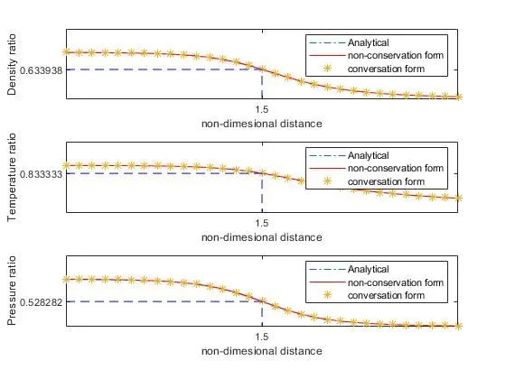
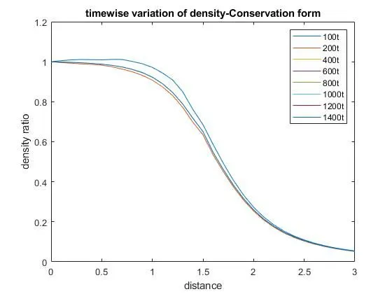
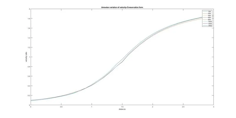
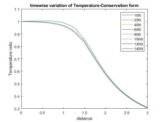
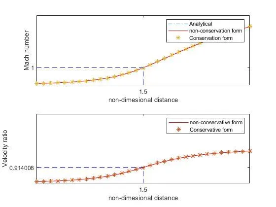
1.comparing a Analytical,non-conservation and conservation form of primitive variables,presence of values in the graph does shows that the difference between these forms are not in the order of `10^-1`
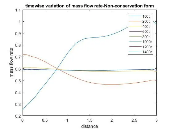
2.while checking timewise variation of non-conservative form of Primitive variables,plot shows a variation after 600 time step it is Converged to the steady state ,At 600 time step even conservative form of primitive variables is converged to the steady state
3.Comparision of Normalised mass flow rate of both forms ,Exact mass flow rate-0.590, where the Conservation form of the plot shows a constant value with minimum fluctuations,where the non-conservation form of Normalised mass flow rate represents that is not a constant from the plot
4.For determining a Normalised mass flow rate,conservation form delivers a better Physical understanding (i.e..,constant or variable )
5.From the program it is clear that both the conversation forms and non-conversation form has converged but not upto accuracy of `10^-9`
I have attached a file link of the file generated to see the grid independence
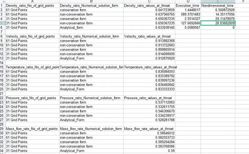
6.From the tabe it is clear non dimensional time stepping 61 grid points is lesser than 31 grid points,this is because of time stepping will decrease when the grid points increasing to retain its stability.
7.from the table we can identify that at 61 grid points,conservation form time stepping is lesser than non-conservation form
8.from the table we can identify that at 31 grid points,non-conservation form time stepping is lesser than conservation form
9.Due to increase in grid points the values changes in the order of `10^-3` which is very small.This factor is taken as grid independence.and non-conservation form is very nearer to the analtyical solution even when we compared with 61 grid point conservation form of primitive variables
10.due to the residuals lesser in non-Consevation form will brings near to the exact value such as analytical for the primitive variables
11.conservation form will brings near to the analytical solution for Flux variables,solution vectors (for mass flow rate )