Week 7 - Simulation of a 1D Super-sonic nozzle flow simulation using Macormack Method
SIMULATION OF A 1D SUBSONIC-SUPERSONIC NOZZLE FLOW USING MACCORMACK METHOD:
OBJECTIVE:
To simulate the isentropic flow through a 1D subsonic-supersonic nozzle by solving the conservation and non-conservation form of governing equations numerically with the help of Macormack method and interpret the results.
PROBLEM STATEMENT:
The given problem is to simulate a 1D subsonic -supersonic nozzle flow using Maccormack method.
In our problem we will simplify the nozzle geometry by considering an area to length relationship as follows:

It can be seen that area is a function of the non-dimensional distance `x`. Here `x=1.5` is the throat, `x<1.5` will be the converging portion and `x>1.5` will be the diverging portion.
Just for simplicity `xprime` which is the actual nondimensional distance is simply denoted as `x` here. `xprime=x/L`, where `x` is the distance along the nozzle and `L` is the length of the nozzle. Also area `A` denoted here is actually a non dimesnional area `Aprime`, which is given by `A/A^**` where `A` is the actual area and `A^**` is the area at the throat. Here `x=1.5` is the throat, `x<1.5` will be the converging portion and `x>1.5` will be the diverging portion. The cross section of the nozzle is shown below:
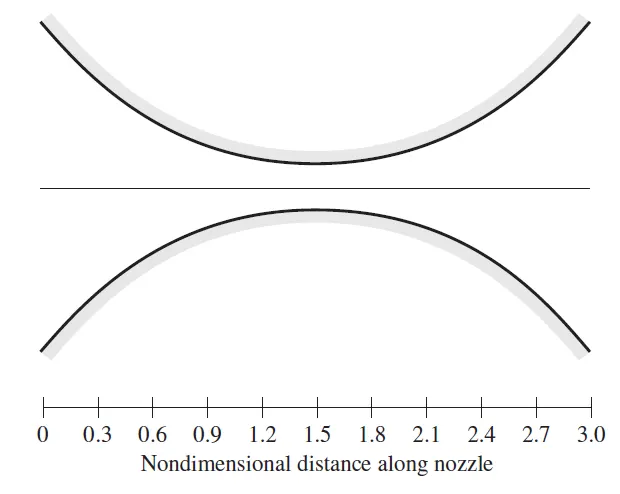
We will simulate the flow through the above nozzle considering both the form of governing equations and compare the results with the analytical solution.
METHODOLOGY:
I. MACCORMACK TECHNIQUE:
In solving the governing equations we use Macormack technique. The Macormack technique is found to be an effecitve tecnique for solving hyperbolic type of equations. The Macormack technique is a two step technique which yields a second order accuracy by taking the average of residue terms(which are of the accurate of first order) in two steps. This can be demonstrated below. Let us consider a simple differential equation as follows:
`(delF)/(delt)=(delF)/(delx)`
If we have an initital condition for the function `F` along the direction `x` we can find the time derivative of `F` in two steps as follows:
1) Predictor step: In the predictor step we do a forward differencing of the RHS and find the residue at the LHS at time `t=0` and at `n`th time step as follows:
`((delF)/(delt))_(i,n)=(F_(i+1,n)-F_(i,n))/(Deltax)`
We use the predicted value for finding the function after a time step `dt` i.e., at `n+1`th time step as follows. We say it as midterm value by denoting a overline on the top of `F`.
`overlineF_(i,n+1)=F_(i,n)+((delF)/(delt))_(i,n)*Deltat`
2) Corrector step: In the corrector step, we do a backward differencing for the RHS at `n+1`th time step with the help of known predicted values from the predictor step, and find the residue of the LHS.
`((delF)/(delt))_(i,n+1)=(overlineF_(i,n+1)-overlineF_(i-1,n))/(Deltax)`
Now we find a average value of the residues of the `n+1`th time step and `n`th time step which can be given by:
`((delF)/(delt))_(ave)=0.5*(((delF)/(delt))_(i,n)+((delF)/(delt))_(i,n+1))`
We use this average value for finding the final value of `F` at the `n+1`th time step by forward differencing ,
`F_(i,n+1)=F_(i,n)+((delF)/(delt))_(ave)*Deltat`
II. SOLVING NON-CONSERVATION FORM OF GOVERNING EQUATION :
The governing equations for the non conservation form of governing equations are shown below:
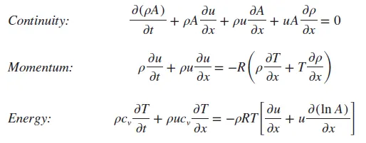
The given equations are non-dimensionalised as follows:
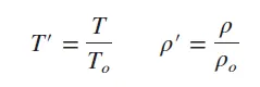
Here `Tprime` and `rhoprime` are non dimensional values for temperature and density, where `T_0` and `rho_0` are the values of temperature and density at the entrance of the nozzle. The length and area are non-dimensionalized as follows as discussed previously:


The velocity `u` is nondimensionalised with the help of speed of sound, `a_0` as follows:

Non dimesnional time is given as follows:
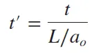
Substituting all the non-dimensional variables we get:



Now we solve this continous, momentum and energy equation with the help of Macormack technique to find the solution at the steady state.
Calculation of time step: For finding the optimum time step, we use a stability criteria for calculation of `Deltat` given by
`Deltat=C.((Deltax)/(a+V))`
where `C` is the courant number `a` is the local speed of sound and `V` is the velocity of the flow. From the CFL criterion, we know the courant number should be less than unity for convergence. In our simulation we have used a courant number of 0.5.
This `Deltat` varies at each node. For our simulation we use minimum of `Deltat` calculated from all the nodes. (t shown here is non dimensional time)

Boundary conditions: A subsonic in-flow condition is considered at the inlet for Velocity with a fixed value of Pressure and temperature is assumed as follows:(`rho`,`V` and `T` are all non-dimensional quantities here)
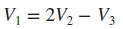
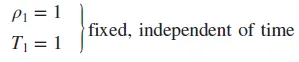
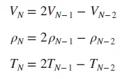
At the exit of the nozzle, supersonice flow boundary condition is maintained for all the three primitive variables:
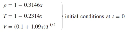
Initial conditions: At `t=0` the initial conditions for the primitive variables are assumed as follows:
With the above explained formulation, we developed a MATLAB user defined function which is attached below. The function will yield outputs such as final steady state values of density, temperature, velocity and pressure. Also the variation of this primitive variables at the throat through out the iterations, final residue and the final non dimensional time are all found.
MATLAB user defined function code for solving Non-conservational form of governing equation:
function [rho,temp,v,p,M,rhot,Mt,Tt,pt,dtdata,tdata,tstep,mflowdata,res,mflow]=solve_nonconserveqn(x,n,gamma,cfl,dx,tstepplot)

% calculate primitive variables i.e at t=0
rho=1-0.3146*x;
temp=1-0.2314*x;
v=(0.1+1.09.*x).*temp.^(1/2);
a=1+2.2*(x-1.5).^2;
rhoold=rho;vold=v;tempold=temp;
t=0;

%Non dimensional pressure and mach number
p=rho.*temp;
M=v./(temp.^0.5);

%obtain the throat value data
rhot(1)=rho((n+1)/2);
Mt(1)=M((n+1)/2);
Tt(1)=temp((n+1)/2);
pt(1)=p((n+1)/2);
dtdata(1)=0;
tdata(1)=t;

%Non dimesnional mass flow rate
mflow=rho.*a.*v;
mflowdata(:,1)=mflow;

%Macormack method solution loop
for tstep=2:1800

%predictor step
for i=2:n-1
drhobydt(i)=-rho(i)*(v(i+1)-v(i))/dx-rho(i)*v(i)*(log(a(i+1))-log(a(i)))/dx-v(i)*(rho(i+1)-rho(i))/dx;
dvbydt(i)=-v(i)*(v(i+1)-v(i))/dx-(1/gamma)*((temp(i+1)-temp(i))/dx+temp(i)/rho(i)*(rho(i+1)-rho(i))/dx);
dtbydt(i)=-v(i)*(temp(i+1)-temp(i))/dx-(gamma-1)*temp(i)*((v(i+1)-v(i))/dx+v(i)*(log(a(i+1))-log(a(i)))/dx);
end
drhobydtold=drhobydt;dvbydtold=dvbydt;dtbydtold=dtbydt;

for i=1:n
dt_all(i)=cfl*(dx/(temp(i)^0.5+v(i)));
end
dt=min(dt_all);

%Mid results
for i=2:n-1
rho(i)=rho(i)+drhobydt(i)*dt;
v(i)=v(i)+dvbydt(i)*dt;
temp(i)=temp(i)+dtbydt(i)*dt;
end

% Apply boundary condidtions
%At first node
v(1)=2*v(2)-v(3); rho(1)=1;temp(1)=1;
%At last node
v(n)=2*v(n-1)-v(n-2);rho(n)=2*rho(n-1)-rho(n-2);
temp(n)=2*temp(n-1)-temp(n-2);

%corrector step-rearward differencing
for i=2:n-1
drhobydt(i)=-rho(i)*(v(i)-v(i-1))/dx-rho(i)*v(i)*(log(a(i))-log(a(i-1)))/dx-v(i)*(rho(i)-rho(i-1))/dx;
dvbydt(i)=-v(i)*(v(i)-v(i-1))/dx-(1/gamma)*((temp(i)-temp(i-1))/dx+temp(i)/rho(i)*(rho(i)-rho(i-1))/dx);
dtbydt(i)=-v(i)*(temp(i)-temp(i-1))/dx-(gamma-1)*temp(i)*((v(i)-v(i-1))/dx+v(i)*(log(a(i))-log(a(i-1)))/dx);
end
%Average of differential elements
for i=2:n-1
drhobydtav(i)=0.5*(drhobydtold(i)+drhobydt(i));
dvbydtav(i)=0.5*(dvbydtold(i)+dvbydt(i));
dtbydtav(i)=0.5*(dtbydtold(i)+dtbydt(i));
end
%Final result
for i=2:n-1
rho(i)=rhoold(i)+drhobydtav(i)*dt;
v(i)=vold(i)+dvbydtav(i)*dt;
temp(i)=tempold(i)+dtbydtav(i)*dt;
end

% Apply boundary condidtions
%At first node
v(1)=2*v(2)-v(3); rho(1)=1;temp(1)=1;
%At last node
v(n)=2*v(n-1)-v(n-2);rho(n)=2*rho(n-1)-rho(n-2);
temp(n)=2*temp(n-1)-temp(n-2);

%Non dimensional pressure and mach number
p=rho.*temp;
M=v./(temp.^0.5);

%Update the time
t=t+dt;

%obtain the throat value data
rhot(tstep)=rho((n+1)/2);
Mt(tstep)=M((n+1)/2);
Tt(tstep)=temp((n+1)/2);
pt(tstep)=p((n+1)/2);
dtdata(tstep)=dt;
tdata(tstep)=t;
mflow=rho.*a.*v;

% Acquire mass flow data at different instances;
if any(tstep==tstepplot)
ind=find(tstepplot==tstep);
mflowdata(:,ind+1)=mflow;
end

%Break the loop if a required accuracy is obtained
res=max([max(abs(rhoold-rho)),max(abs(tempold-temp)),max(abs(vold-v))]);
if res<10^-10
    break;
end

% Re-allocate the values
rhoold=rho;vold=v;tempold=temp;
end

end
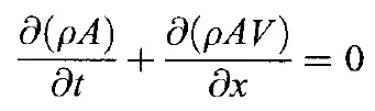
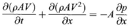
III. SOLVING CONSERVATION FORM OF GOVERNING EQUATION :
The governing equations for the conservation form of governing equations are shown below:
Continuity:
Momentum:
Energy:

The non-dimensionalisation of the above governing equations yields as follows:
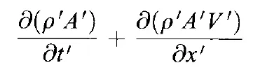


In order to simplify the above equations we will convert them into a generic form by the substititutions as follows:
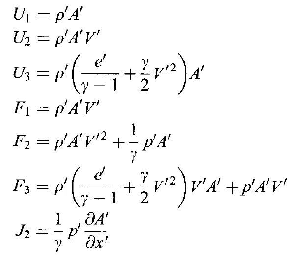
Then the substituted equations becomes as:
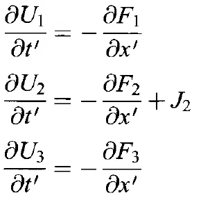
This will be the final equation which we will use in Macormack technique.
At each time step we will decode our primitive variables from the unknown vectors as follows:
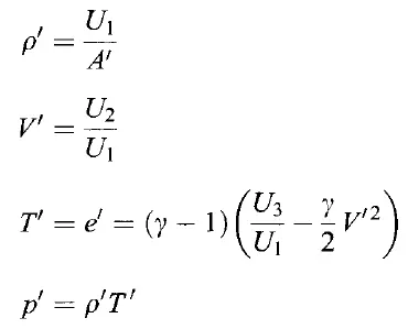
The flux term and the source term in the RHS of the governing equation can be found by
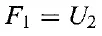
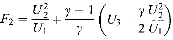
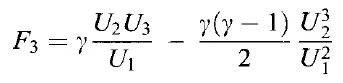
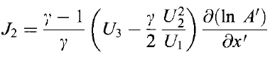
Calculation of time step: The calculation of time step will be done in a similar procedure as we did in solving non-conservation form of governing equation.
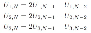
Boundary condition: The boundary conditions are given in such a way that the inflow has a subsonic flow and the outflow has a supersonic flow which are given as follows:
Inlet conditions:


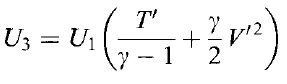
Exit conditions:
Initial conditions: The intial conditions are assumed in such a way to obtain the solution quicker as from the reference of John Anderson, Computational Fluid dynamics book.
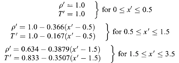
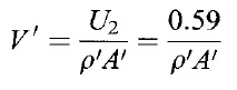
With the above explained formulation, we developed a MATLAB user defined function which is attached below.
MATLAB user defined function code for solving conservational form of governing equation:
function [rho,temp,v,p,M,rhot,Mt,Tt,pt,dtdata,tdata,tstep,mflowdata,res,mflow]=solve_conserveqn(x,n,gamma,cfl,dx,tstepplot)

% calculate primitive variables i.e at t=0
a=1+2.2*(x-1.5).^2; %Area
t=0;
% INITITAL CONDITIONS: Calculate primitive variables i.e at t=0
p1=find(x==0.5);p2=find(x==1.5);p3=find(x==3);
for i=1:p1
rho(i)=1;
temp(i)=1;
end
for i=p1+1:p2
rho(i)=1-0.366*(x(i)-0.5);
temp(i)=1-0.167*(x(i)-0.5);
end
for i=p2+1:p3
rho(i)=0.634-0.3879*(x(i)-1.5);
temp(i)=0.833-0.3507*(x(i)-1.5);
end
v=0.59./(rho.*a);

%Solution vector at initial conditions
u1=rho.*a; u2=rho.*a.*v; u3=rho.*(temp./(gamma-1)+(gamma/2)*v.^2).*a;

%Non dimensional pressure and mach number
p=rho.*temp;
M=v./(temp.^0.5);
%obtain the throat value data
rhot(1)=rho((n+1)/2);
Mt(1)=M((n+1)/2);
Tt(1)=temp((n+1)/2);
pt(1)=p((n+1)/2);
dtdata(1)=0;
tdata(1)=t;
mflowdata(:,1)=u2;

for tstep=2:1800
u1old=u1;u2old=u2;u3old=u3;

%Predictor step
f1=u2; f2=((u2.^2)./u1+((gamma-1)/gamma).*(u3-(gamma/2).*((u2.^2)./u1)));
f3=gamma.*u2.*u3./u1-(gamma*(gamma-1)/2).*(u2.^3)./(u1.^2);
for i=2:n-1
j2(i)=(1/gamma)*rho(i)*temp(i)*(a(i+1)-a(i))/dx;
end

%calculate forward difference
for i=2:n-1
du1bydt(i)=-(f1(i+1)-f1(i))/dx;
du2bydt(i)=-(f2(i+1)-f2(i))/dx+j2(i);
du3bydt(i)=-(f3(i+1)-f3(i))/dx;
end
du1bydtold=du1bydt;du2bydtold=du2bydt;du3bydtold=du3bydt;

% Calculate minimum time step
dt_all=cfl*(dx./(temp.^0.5+v));
dt=min(dt_all);

%calculate mid values at t+dt
for i=2:n-1
u1(i)=u1(i)+du1bydt(i)*dt;
u2(i)=u2(i)+du2bydt(i)*dt;
u3(i)=u3(i)+du3bydt(i)*dt;
end

% boundary conditions
u1(1)=a(1); u2(1)=2*u2(2)-u2(3);u3(1)=u1(1)*(1/(gamma-1)+(gamma/2)*v(1)^2);
u1(n)=2*u1(n-1)-u1(n-2);u2(n)=2*u2(n-1)-u2(n-2);u3(n)=2*u3(n-1)-u3(n-2);

% Reassign mid term primitive variables and unknown vector at t+dt
rho=u1./a;
temp=(gamma-1).*(u3./u1-(gamma/2).*(u2./u1).^2);
f1=u2; f2=((u2.^2)./u1+((gamma-1)/gamma).*(u3-(gamma/2).*((u2.^2)./u1)));
f3=gamma.*u2.*u3./u1-(gamma*(gamma-1)/2).*(u2.^3)./(u1.^2);
for i=2:n-1
j2(i)=(1/gamma)*rho(i)*temp(i)*(a(i)-a(i-1))/dx;
end

% %corrector step-REarward difference
for i=2:n-1
% j2(i)=(1/gamma)*rho(i)*temp(i)*(a(i+1)-a(i))/dx;
du1bydt(i)=-(f1(i)-f1(i-1))/dx;
du2bydt(i)=-(f2(i)-f2(i-1))/dx+j2(i);
du3bydt(i)=-(f3(i)-f3(i-1))/dx;
end
%
%average time derivative
du1bydtav=0.5*(du1bydt+du1bydtold);
du2bydtav=0.5*(du2bydt+du2bydtold);
du3bydtav=0.5*(du3bydt+du3bydtold);
%
%final solution vector
for i=2:n-1
u1(i)=u1old(i)+du1bydtav(i)*dt;
u2(i)=u2old(i)+du2bydtav(i)*dt;
u3(i)=u3old(i)+du3bydtav(i)*dt;
end
% boundary conditions
u1(1)=a(1); u2(1)=2*u2(2)-u2(3);u3(1)=u1(1)*(1/(gamma-1)+(gamma/2)*v(1)^2);
u1(n)=2*u1(n-1)-u1(n-2);u2(n)=2*u2(n-1)-u2(n-2);u3(n)=2*u3(n-1)-u3(n-2);

%final primitive variables
% for i=2:n-1
rho=u1./a;
v=u2./u1;
temp=(gamma-1).*(u3./u1-(gamma/2).*v.^2);

%Non dimensional pressure and mach number
p=rho.*temp;
M=v./(temp.^0.5);
mflow=u2;

t=t+dt;

%obtain the throat value data
rhot(tstep)=rho((n+1)/2);
Mt(tstep)=M((n+1)/2);
Tt(tstep)=temp((n+1)/2);
pt(tstep)=p((n+1)/2);
dtdata(tstep)=dt;
tdata(tstep)=t;

% Acquire mass flow data at different instances;
if any(tstep==tstepplot)
ind=find(tstepplot==tstep);
mflowdata(:,ind+1)=mflow;
end

%Break the loop if a required accuracy is obtained
res=max([max(abs(u2old-u2)),max(abs(u1old-u1)),max(abs(u3old-u3))]);
if res<10^-10
    break;
end

end
Other conditions while running the simulation while solving both the form of governing equations:
The solution was stopped if the maximum of all the residuals of the primitive variables was below less than `10^-10`. Otherwise the iterations will stop at a maximum number of 1800 and report the results.
III.ANALYTICAL SOLUTION
The analytical solution can be readily obtained by solving the governing equations analytically. The solution equations from the reference of the John Anderson, CFD book is given below:

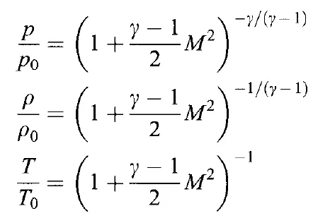
The above four relations will be used for finding the Mach number, pressure relation, density relation and temperature relation respectively.
MATLAB user defined function code for finding the analytical solution:
The relations are used to find the property values at each node with the help of MATLAB functions as follows:
% ANALYTICAL SOLUTION
function [M,pdash, rhodash,Tdash]=solve_analytical(x,g)
for i=1:(length(x)+1)/2
    a=1+2.2*(x(i)-1.5)^2;
fun = @(M)((1/M^2)*((2/(g+1))*(1+(g-1)/2*M^2))^((g+1)/(g-1))-a^2);
M0 = 1;
M(i) = fzero(fun,M0);
end
for i=(length(x)+1)/2+1
    a=1+2.2*(x(i)-1.5)^2;
fun = @(M)((1/M^2)*((2/(g+1))*(1+(g-1)/2*M^2))^((g+1)/(g-1))-a^2);
M0 = 1.5;
M(i) = fzero(fun,M0);
end
for i=(length(x)+1)/2+2:length(x)
    a=1+2.2*(x(i)-1.5)^2;
fun = @(M)((1/M^2)*((2/(g+1))*(1+(g-1)/2*M^2))^((g+1)/(g-1))-a^2);
M0 = 2;
M(i) = fzero(fun,M0);
end

%Finding primitive variables
pdash=(1+((g-1)/2).*M.^2).^(-g/(g-1));
rhodash=(1+((g-1)/2).*M.^2).^(-1/(g-1));
Tdash=(1+((g-1)/2).*M.^2).^(-1);
end
IV INTERPRETATION OF RESULTS
All the function files are called from a general code and the required results are interpreted. The MATLAB code is attached below:
%% CFD SOLUTION OF SUBSONIC-SUPERSONIC ISENTROPIC NOZZLE FLOW:MACCOMARCK...
%...TECHNIQUE
clc
clear all
close all

%% COMMON INPUTS-Grid size and problem constants
n=31; % Change Number of nodes to study grid independence study;Tried values are 31,61,91
x=linspace(0,3,n);
dx=x(2)-x(1);
gamma=1.4;
cfl=0.5;
tstepplot=[100,200,400,700,1000];

%% SOLVING NON-CONSERVATION FORM OF GOVERNING EQUATION

[rho,temp,v,p,M,rhot,Mt,Tt,pt,dtdata,tdata,tstep,mflowdata,res,mflowfinal]=solve_nonconserveqn(x,n,gamma,cfl,dx,tstepplot);

%PRINT OUTPUT
fprintf('\nOUTPUT\n')
if res<=10^-10
fprintf(['\nThe solution from solving non-conservational form of governing equation is obtained after %d iterations \n..' ...
    'with a maximum residual of %e'],tstep,res);

elseif res>10^-10
  fprintf(['\nThe iteration is stopped after a maximum %d iterations for solving non-conservational form of governing equation\n..' ...
    'the maximum residual obtained was %e\n'],tstep,res);
end

%PLOT OUTPUT FOR NON-CONSERVATION FORM OF GOVERNING EQUATION
%Plotting Timewise variation of primitive variables and Mach number at the nozzle throat
figure;
nsteps=(1:tstep);
subplot(4,1,1)
plot(nsteps,rhot);
ylabel('Density ratio')
title('Timewise variation of primitive variables and Mach number at the nozzle throat','Solving Nonconservation form of governing Equations')
subplot(4,1,2)
plot(nsteps,Tt);
ylabel('Temperature ratio')
subplot(4,1,3)
plot(nsteps,pt);
ylabel('Pressure ratio')
subplot(4,1,4)
plot(nsteps,Mt);
ylabel('Mach number')
xlabel('Number of time steps')

%Plotting steady state distributions of primitive variables and Mach number inside the nozzle
figure;
subplot(4,1,1)
plot(x,M);
ax=gca;
ax.YAxis.TickLabelFormat = '%0.1f';
ylabel('Mach number')
title('Steady state distributions of primitive variables and Mach number inside the nozzle','Solution for Nonconservation form of governing Equations')
subplot(4,1,2)
plot(x,p);
ylabel('Pressure ratio')
subplot(4,1,3)
plot(x,rho);
ylabel('Density ratio')
subplot(4,1,4)
plot(x,temp);
ylabel('Temperature ratio')
xlabel('Distance through nozzle (x)')

%Plotting Instantaneous mass flow distribution at various time steps
figure;
f=plot(x,mflowdata);
f(1).LineWidth = 1.5;f(1).Color = 'k';f(1).LineStyle = '--';f(6).LineWidth = 1.5;
legend('0\Deltat','100\Deltat','200\Deltat','400\Deltat','700\Deltat','1000\Deltat')
ylabel('Non-dimensional mass flow')
xlabel('Distance through nozzle (x)')
title('Instantaneous distributions of non-dimensional mass flow as a function of distance through nozzle at different times','Solution of Nonconservation form of governing Equations')

%% SOLVING CONSERVATION FORM OF GOVERNING EQUATION

[rhoc,tempc,vc,pc,Mc,rhotc,Mtc,Ttc,ptc,dtdatac,tdatac,tstepc,mflowdatac,resc,mflowfinalc]=solve_conserveqn(x,n,gamma,cfl,dx,tstepplot);

%PRINT OUTPUT
if resc<=10^-10
fprintf(['\nThe solution from solving conservational form of governing equation is obtained after %d iterations \n..' ...
    'with a maximum residual of %e'],tstepc,resc);

elseif resc>10^-10
  fprintf(['\nThe iteration is stopped after a maximum %d iterations for solving conservational form of governing equation\n..' ...
    'the maximum residual obtained was %e\n'],tstepc,resc);
end

%PLOT OUTPUT FOR CONSERVATION FORM OF GOVERNING EQUATION
%Plotting Timewise variation of primitive variables and Mach number at the nozzle throat
figure;
nsteps=1:tstepc;
subplot(4,1,1)
plot(nsteps,rhotc);
ylabel('Density ratio')
title('Timewise variation of primitive variables and Mach number at the nozzle throat','Solving conservation form of governing Equations')
subplot(4,1,2)
plot(nsteps,Ttc);
ylabel('Temperature ratio')
subplot(4,1,3)
plot(nsteps,ptc);
ylabel('Pressure ratio')
subplot(4,1,4)
plot(nsteps,Mtc);
ylabel('Mach number')
xlabel('Number of time steps')

%Plotting steady state distributions of primitive variables and Mach number inside the nozzle
figure;
subplot(4,1,1)
plot(x,Mc);
ax=gca;
ax.YAxis.TickLabelFormat = '%0.1f';
ylabel('Mach number')
title('Steady state distributions of primitive variables and Mach number inside the nozzle','Solution for conservation form of governing Equations')
subplot(4,1,2)
plot(x,pc);
ylabel('Pressure ratio')
subplot(4,1,3)
plot(x,rhoc);
ylabel('Density ratio')
subplot(4,1,4)
plot(x,tempc);
ylabel('Temperature ratio')
xlabel('Distance through nozzle (x)')

%Plotting Instantaneous mass flow distribution at various time steps
figure;
f=plot(x,mflowdatac);
f(1).LineWidth = 1.5;f(1).Color = 'k';f(1).LineStyle = '--';f(6).LineWidth = 1.5;
legend('0\Deltat','100\Deltat','200\Deltat','400\Deltat','700\Deltat','1000\Deltat')
ylabel('Nondimensional mass flow')
xlabel('Distance through nozzle (x)')
title('Instantaneous distributions of non-dimensional mass flow as a function of distance through nozzle at different times','Solution of conservation form of governing Equations')

%% ANALYTICAL SOLUTION
[Ma,pa, rhoa,Ta]=solve_analytical(x,gamma);
a=1+2.2*(x-1.5).^2; %Area
velocity=Ma.*Ta.^0.5;
mflowa=rhoa.*a.*velocity;

%PLOT OUTPUT FOR ANALYTICAL SOLUTION
%Plotting steady state distributions of primitive variables and Mach number
%inside the nozzle for Analytical solution
figure;
subplot(4,1,1)
plot(x,Ma);
ax=gca;
ax.YAxis.TickLabelFormat = '%0.1f';
ylabel('Mach number')
title('Steady state distributions of primitive variables and Mach number inside the nozzle','Analytical solution')
subplot(4,1,2)
plot(x,pa);
ylabel('Pressure ratio')
subplot(4,1,3)
plot(x,rhoa);
ylabel('Density ratio')
subplot(4,1,4)
plot(x,Ta);
ylabel('Temperature ratio')
xlabel('Distance through nozzle (x)')

%% COMPARISON OF SOLUTION OF DIFFERENT FORM OF GOVERNING EQUATIONS WITH ANALYTICAL SOLUTION
%Comparing the final steady state mass flow distribution for different form of governing equation with analytical result
figure;
plot(x,mflowfinal,x,mflowfinalc,x,mflowa);
ylabel('Nondimensional mass flow')
xlabel('Distance through nozzle (x)')
legend('Non-conservation form','Conservation form','Analytical solution')
title('Non-dimensional mass flow distribution','Comparison of solution of different form of governing equations with analytical solution')
Output:
Initially 31 nodes will be considered. The output will show whether the solution is converged or not with the maximum residual at the end of time step. The output for the number of nodes of 31 is given below:

Convergence:
We set a maximum residual of `10^-10` for the convergence. From the output we can see that the solution for the non-conservational form of governing equation converged at 1665 number of iterations whereas, the solution for solving conservational form of governing equation was obtained with a residue of `~10^-6` for the maximum number of iterations of 1800.
Timewise variation of primitive variables:
The timewise variation of primitive variables are studied at the nozzle throat for both the governing equation. The output is shown below:
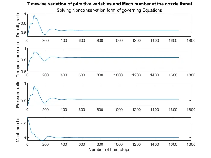
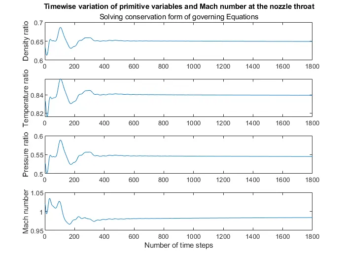
It can be seen that, after a 800 number of time steps there is no flucutation in the primitive variables at the throat while solving both the form of governing equation.
Steady state variation of primitive variables through the nozzle at the end of time step:
Though the solution of non-conservation form of governing equation is converged based on our convergence criteria of `10^-10`, the solution for conservation form of governing equation with a residue of `10^-6` is considered to be steady and the final result is shown below:
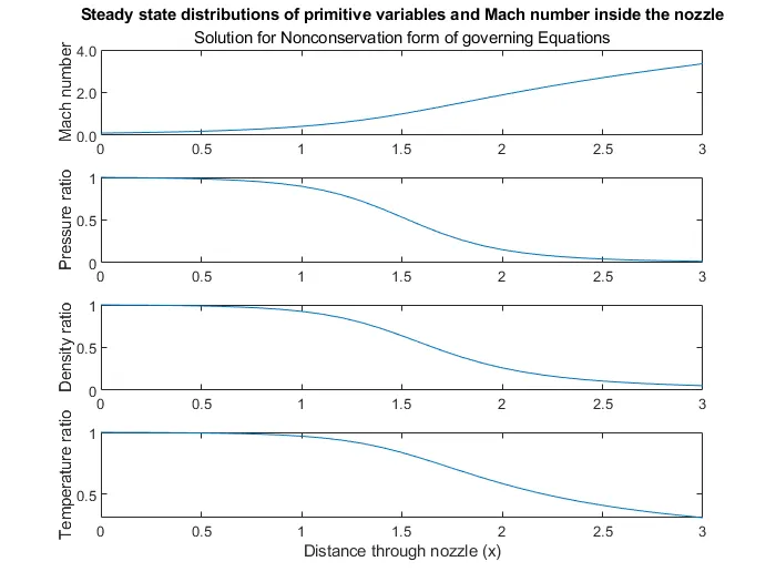
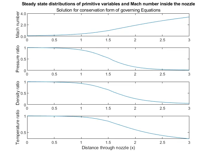
It can be seen that both the plots are almost similar. Now we will compare the above results with the analytical solution below:
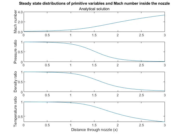
It can be seen that the analytical solution is also similar. So our results are qualitatively satisfactory.
Variation of mass flow distribution through the nozzle at different time step:
Since our initial conditions while solving each form of governing equation is different, we will see individually the variation of mass distributions for different form of governing equation.
Non-conservational form of governing equation:
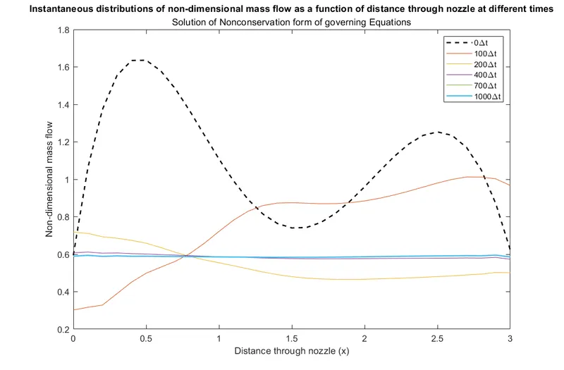
Initial condition is shown here in dark dashed black colour and the solution after 1000 time steps is shown in light blue line(since we know that the variations are negligible after 1000 time step). It can be seen that the mass flow rate is almost constant throughout the nozzle.
Conservational form of governing equation:
A similar pattern is observed for the conservational form of governing equation which is shown below:
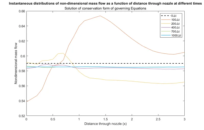
Though our initial condition is constant throughout the nozzle, there was a fluctuation in between and finally a constant solution is obtained.
Comparison of the final solution of both the form of governing equation with the analytical solution:
The final mass flow distribution is compared and shown below:
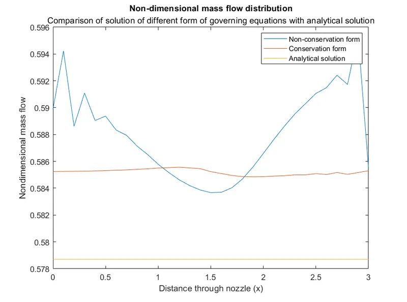
It can be seen that the analytical solution yielded a constant mass flow inside the nozzle with a non-dimesnional value of 0.5787. Our solution from the conservation form yielded a mass flow which is almost constant with an error of around `10^-3`. However the solution of non-conservation form of governing equation is not constant throughout the nozzle and the variation was within `10^-2`which might be acceptable in most of the cases.
Grid independence study:
The grid size is changed from 31 nodes to 61 nodes and 91 nodes and the results are studied.
1) For 61 nodes:
The following output was obtained:

Both the form of governing equation yielded a maximum residual of `~10^-7`. Eventhough the results look satisfactory, both the form of governing equation did not satisfy our convergence criteria i.e.,`10^-10`.
We obtained a similar profile for the primitive variable. The final mass ditributions is compared and shown below:
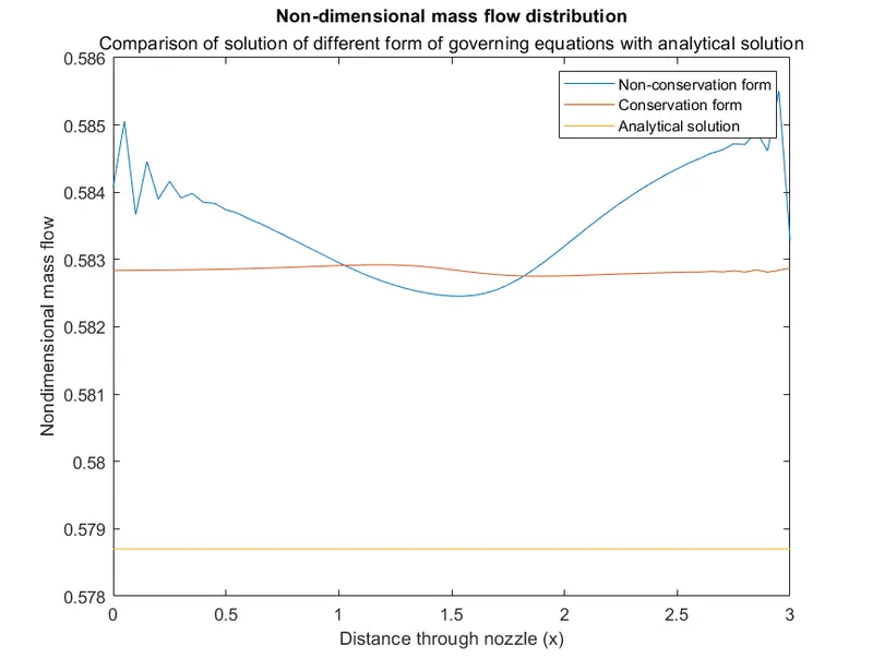
The results were similar to the result with 31 nodes, however the result with non-conservational form of governing equation is improved with less fluctuation compared to the previous one. Although both the results deviated from the analytical solution upto an error of ~0.006.
2) For 91 nodes:
The following output was obtained:

Both the form of governing equation yielded a maximum residual of `~10^-5`. The value of the residue is further reduced. The increase in the final number of time steps may yield a better result, however considering the computational time, the iteration is stopped.
We obtained a similar profile for the primitive variable. The final mass ditributions is compared and shown below:
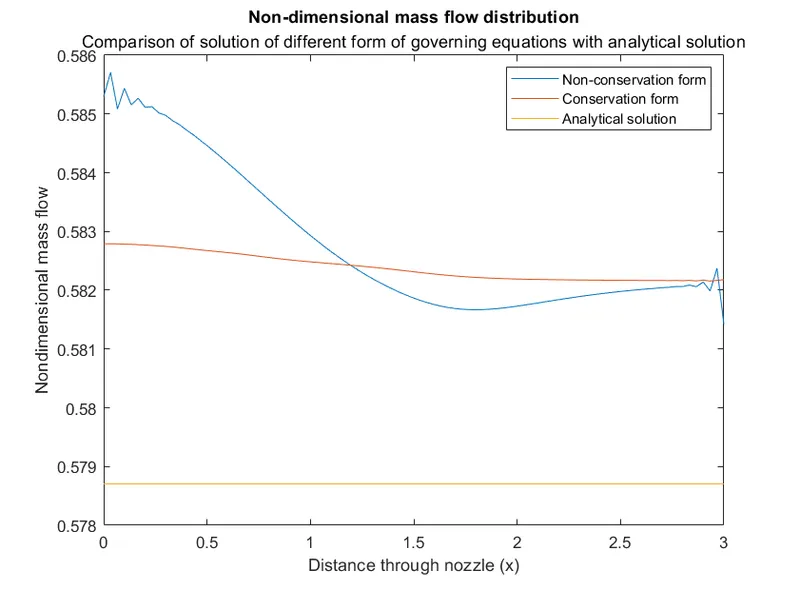
We observed a similar profile as in the previous case and it was found that the increase in number of nodes did not increase the performace of results quantitatively for the mass distributions.
CONCLUSION:
1) Solving non conservation form of governing equation yielded a good result for the primitive variables, while conservation form of governing equation yielded a good result for the mass distribution. This is because the conservation form of governing equation conserved the mass flow during the simulation.
2) Both the form of governing equation yielded a satisfactory result. However, solving the conservation form of governing equation is little tedious which involves a number of alterations in the governing equations.
3) From the grid independence study it was observed that, increasing the grid size increased the computational time. However the results are not changed significantly. Hence a 31 number of nodes can be found to be satisfactory for the given problem.