Week 3.5 - Deriving 4th order approximation of a 2nd order derivative using Taylor Table method

Deriving 4th order approximation of a 2nd order derivative using Taylor Table method

The given function is `u=f(x)=exp(x)*cos(x)`. We have to find the fourth order approximation of the second order derivative of the function using different schemes as follows:

1. Central difference

2. Skewed right-sided difference

3. Skewed left-sided difference

Also we have to find the error with respect to the analytical derivative at a given `x` for each of these scheme and we have to find how these errors are dependent on the value of the space discretization `dx`.

Step 1: Find the analytical derivative of the given function:

By differentiating the given function for two times we get:

`f''(x)=-2*exp(x).*sin(x)`

Step 2: Find the discretization formula for different schemes:

1) Central difference scheme

First we will find the formula for Central difference scheme. We need to know the number of nodes to be used which we can find from the below formula:

The order of accuracy P = Number of nodes in the stencil N - order of derivative Q + 1 for symmetric/central schemes----(i)

Here,

Q = 2 for second order derivative

P = 4 for fourth order accuracy

Now substituting in (i) we get N = 5 (Number of nodes to be considered)

So if we consider a node at `x=i`, we can consider two neighbouring nodes on both sides for achieving the required order of accuracy.

So the stencil may look like:

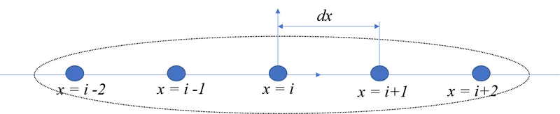
We can represent the central differencing scheme of the second order derivative as:

`((Deltax)^2(d^2u)/dx^2)_(x=i) cong a.f(i-2)+b.f(i-1)+c.f(i)+d.f(i+1)+e.f(i+2)` --------- `(I)`

Now we construct the Taylor's table considering the given number of nodes:

	`f(i)`	`Deltax.f'(i)`	`(Deltax)^2.f''(i)`	`(Deltax)^3.f^((iii))(i)`	`(Deltax)^4.f^((iv))(i)`	`(Deltax)^5.f^((v))(i)`	`(Deltax)^6.f^((vi))(i)`
`a.f(i-2)`	`a`	`(-2)a`	`((-2)^2.a)/(2!)`	`((-2)^3.a)/(3!)`	`((-2)^4.a)/(4!)`	`((-2)^5.a)/(5!)`	`((-2)^6.a)/(6!)`
`b.f(i-1)`	`b`	`(-1)b`	`((-1)^2.b)/(2!)`	`((-1)^3.b)/(3!)`	`((-1)^4.b)/(4!)`	`((-1)^5.b)/(5!)`	`((-1)^6.b)/(6!)`
`c.f(i)`	`c`	`0`	`0`	`0`	`0`	`0`	`0`
`d.f(i+1)`	`d`	`d`	`((1)^2.d)/(2!)`	`((1)^3.d)/(3!)`	`((1)^4.d)/(4!)`	`((1)^5.d)/(5!)`	`((1)^6.d)/(6!)`
`e.f(i+2)`	`e`	`2e`	`((2)^2.e)/(2!)`	`((2)^3.e)/(3!)`	`((2)^4.e)/(4!)`	`((2)^5.e)/(5!)`	`((2)^6.e)/(6!)`
	`(1)`	`(2)`	`(3)`	`(4)`	`(5)`	`(6)`	`(7)`

Here column `(1)` represents coefficients of `f(x)`, `(2)` represents coefficients of `Deltax.f'(x)` and so on for the weighted value of the function at each node such as `a.f(i-2)` , `b.f(i-1)`, etc.,

Now in order to find the weights `a, b, c, d` and `e` (5 unknowns) we may need 5 equations. So, we will equate the sum of coefficients from column `(1)` to `(5)`with the coefficients in L.H.S .i.e., `((Deltax)^2(d^2u)/dx^2)_(x=i)`

All the other coefficients are zero except for `(Deltax)^2.f''(i)` which is equal to one. Now we write the equations in matrix form as:

`AX=B` where

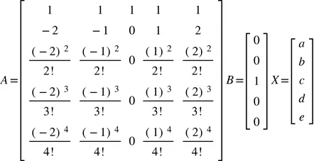
The weights are found with the help of MATLAB code as follows

clear
close all
clc

f2=factorial(2);
f3=factorial(3);
f4=factorial(4);
f5=factorial(5);
f6=factorial(6); 

A=[1 1 1 1 1;
   -2 -1 0 1 2;
   (-2)^2/f2 (-1)^2/f2 0 1/2 2^2/2;
   (-2)^3/f3 (-1)^3/f3 0 1/f3 2^3/f3;
   (-2)^4/f4 (-1)^4/f4 0 1/f4 2^4/f4];
b=[0;0;1;0;0];

format rat
X=A\b
c=[2^6/f6 1/f6 0 1/f6 2^6/f6]*X

We have chosen the output value to be a rational value in order to reduce the round off error. The output is attached here:

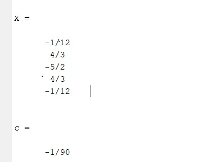
Here the MATLAB output `c` is the sum of coefficients in the column (7). The weights are as follows:

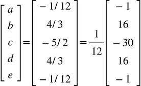
Here the MATLAB output `c` is the sum of coefficients in the column (7).

To prove that the order of approximation is fourth order, we can find the sum of coefficients in `(6)` and `(7)`.

The sum of coefficients in `(6)` becomes zero since `b=d and a=e` and the sum of coefficients in `(7)` was obtained from the output shown previously which is `-1/90`. Also we know sum of coefficients in `(1), (2), (4) and (5)` are zero except for `(3)` which is one.

So, expanding the Taylor's table we can get

`((Deltax)^2(d^2u)/dx^2)_(x=i) cong a.f(i-2)+b.f(i-1)+c.f(i)+d.f(i+1)+e.f(i+2)=`

`0 + 0 + (Deltax)^2.f''(i) + 0 +0 + (-1/90)(Deltax)^6.f^((vi))(i) + . . ."Higher order terms"`

Dividing throughout by `(Deltax)^2 ` we get

`((d^2u)/dx^2)_(x=i) cong (a.f(i-2)+b.f(i-1)+c.f(i)+d.f(i+1)+e.f(i+2))/(Deltax)^2=`

`0 + 0 + f''(i) + 0 +0 + (-1/90)(Deltax)^4.f^((vi))(i) + . . ."Higher order terms"`

So it can be seen that the L.H.S will be our required approximation with the error of the order of `(Deltax)^4`

Now substituting the weights such as `a, b, c, d` and `e` in the equation `(I)` we get

`((d^2u)/dx^2)_(x=i) cong (-f(i-2)+16f(i-1)-30f(i)+16f(i+1)-f(i+2))/(12(Deltax)^2)` ------ (Take it as)--`(II)`

2) Skewed Right sided differencing Scheme:

First we need to know the number of nodes to be used which we can find from the below fomula:

The order of accuracy P = Number of nodes in the stencil N - order of derivative Q for asymmetric/skewed schemes----(ii)

Here,

Q = 2 for second order derivative

P = 4 for fourth order accuracy

Now substituting in (i) we get N = 6 (Number of nodes to be considered)

So if we consider a node at `x=i`, and we can consider five neighbouring nodes on right sides for achieving the required order of accuracy.

So the stencil may look like:

Now we can represent the skewed right sided scheme of the second order derivative as:

`((Deltax)^2(d^2u)/dx^2)_(x=i) cong a.f(i)+b.f(i+1)+c.f(i+2)+d.f(i+3)+e.f(i+4) +f.f(i+5)` --------- `(III)`

Now we can construct the Taylor's table considering the given number of nodes:

	`f(i)`	`Deltax.f'(i)`	`(Deltax)^2.f''(i)`	`(Deltax)^3.f^((iii))(i)`	`(Deltax)^4.f^((iv))(i)`	`(Deltax)^5.f^((v))(i)`	`(Deltax)^6.f^((vi))(i)`
`a.f(i)`	`a`	`0`	`0`	`0`	`0`	`0`	`0`
`b.f(i+1)`	`b`	`b`	`(b)/(2!)`	`(b)/(3!)`	`(b)/(4!)`	`(b)/(5!)`	`(b)/(6!)`
`c.f(i+2)`	`c`	`2c`	`((2)^2.c)/(2!)`	`((2)^3.c)/(3!)`	`((2)^4.c)/(4!)`	`((2)^5.c)/(5!)`	`((2)^6.c)/(6!)`
`d.f(i+3)`	`d`	`3d`	`((3)^2.d)/(2!)`	`((3)^3.d)/(3!)`	`((3)^4.d)/(4!)`	`((3)^5.d)/(5!)`	`((3)^6.d)/(6!)`
`e.f(i+4)`	`e`	`4e`	`((4)^2.e)/(2!)`	`((4)^3.e)/(3!)`	`((4)^4.e)/(4!)`	`((4)^5.e)/(5!)`	`((4)^6.e)/(6!)`
`f.f(i+5)`	`f`	`5f`	`((5)^2.f)/(2!)`	`((5)^3.f)/(3!)`	`((5)^4.f)/(4!)`	`((5)^5.f)/(5!)`	`((5)^6.f)/(6!)`
	`(1)`	`(2)`	`(3)`	`(4)`	`(5)`	`(6)`	`(7)`

Now in order to find the weights `a, b, c, d, e` and `f` (6 unknowns) we may need 6 equations. So, we will equate the sum of coefficients from column `(1)` to `(6)`with the coefficients in L.H.S .i.e., `((Deltax)^2(d^2u)/dx^2)_(x=i)`

All the other coefficients are zero except for `(Deltax)^2.f''(i)` which is equal to one. Now we write the equations in matrix form as:

`AX=B` where

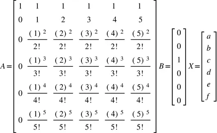
The weights are found with the help of matlab as follows

A1=[1 1 1 1 1 1;
    0 1 2 3 4 5;
    0 1/2 2^2/2 3^2/2 4^2/2 5^2/2;
    0 1/f3 2^3/f3 3^3/f3 4^3/f3 5^3/f3;
    0 1/f4 2^4/f4 3^4/f4 4^4/f4 5^4/f4;
    0 1/f5 2^5/f5 3^5/f5 4^5/f5 5^5/f5];
b1=[0; 0; 1; 0; 0; 0];

X1=A1\b1
c1=[0 1/f6 2^6/f6 3^6/f6 4^6/f6 5^6/f6]*X1

The above code was written as the continuation of the previous code. Hence the output will be in rational value which is attached below

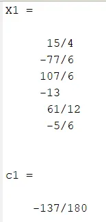
Hence the weights are

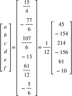
Here the output `c1` is the sum of coefficients in the column (7)

To prove that the order of approximation is fourth order, we can substitute the weights and find the sum of coefficients of `(7)`. It was found already from MATLAB output as `-137/180`.

We know sum of coefficients in `(1), (2), (4) ,(5)` and `(6)` are zero except `(3)` which is one.

So, expanding the Taylor's table we can get

`((Deltax)^2(d^2u)/dx^2)_(x=i) cong a.f(i)+b.f(i+1)+c.f(i+2)+d.f(i+3)+e.f(i+4) +f.f(i+5)=`

`0 + 0 + (Deltax)^2.f''(i) + 0 +0 + 0+(-137/180)(Deltax)^6.f^((vi))(i) + . . ."Higher order terms"`

Dividing throughout by `(Deltax)^2 ` we get

`((d^2u)/dx^2)_(x=i) cong (a.f(i)+b.f(i+1)+c.f(i+2)+d.f(i+3)+e.f(i+4) +f.f(i+5))/(Deltax)^2`

`=0 + 0 + f''(i) + 0 +0 + (-137/180)(Deltax)^4.f^((vi))(i) + . . ."Higher order terms"`

So, it can be seen that the L.H.S will be our required approximation with the error of the order of `(Deltax)^4`

Now substituting the weights such as `a, b, c, d` and `e` in the equation `(III)` we get

`((d^2u)/dx^2)_(x=i) cong (45f(i)-154f(i+1)+214f(i+2)-156f(i+3)+61f(i+4) -10f(i+5))/(12(Deltax)^2)` ------ (Take it as)--`(IV)`

3) Skewed Left sided differencing Scheme:

The number of nodes will be same as that of the right handed scheme, however we have to consider five neighbouring nodes on left hand side of `x=i`

So the stencil may look like:

Now we can represent the skewed left sided differencing scheme of the second order derivative as:

`((Deltax)^2(d^2u)/dx^2)_(x=i) cong a.f(i-5)+b.f(i-4)+c.f(i-3)+d.f(i-2)+e.f(i-1) +f.f(i)` --------- `(V)`

Now we can construct the Taylor's table considering the given number of nodes:

	`f(i)`	`Deltax.f'(i)`	`(Deltax)^2.f''(i)`	`(Deltax)^3.f^((iii))(i)`	`(Deltax)^4.f^((iv))(i)`	`(Deltax)^5.f^((v))(i)`	`(Deltax)^6.f^((vi))(i)`
`a.f(i-5)`	`a`	`a(-5)`	`((-5)^2.a)/(2!)`	`((-5)^3.a)/(3!)`	`((-5)^4.a)/(4!)`	`((-5)^5.a)/(5!)`	`((-5)^6.a)/(6!)`
`b.f(i-4)`	`b`	`b(-4)`	`((-4)^2.b)/(2!)`	`((-4)^3.b)/(3!)`	`((-4)^4.b)/(4!)`	`((-4)^5.b)/(5!)`	`((-4)^6.b)/(6!)`
`c.f(i-3)`	`c`	`c(-3)`	`((-3)^2.c)/(2!)`	`((-3)^3.c)/(3!)`	`((-3)^4.c)/(4!)`	`((-3)^5.c)/(5!)`	`((-3)^6.c)/(6!)`
`d.f(i-2)`	`d`	`d(-2)`	`((-2)^2.d)/(2!)`	`((-2)^3.d)/(3!)`	`((-2)^4.d)/(4!)`	`((-2)^5.d)/(5!)`	`((-2)^6.d)/(6!)`
`e.f(i-1)`	`e`	`e(-1)`	`((-1)^2.e)/(2!)`	`((-1)^3.e)/(3!)`	`((-1)^4.e)/(4!)`	`((-1)^5.e)/(5!)`	`((-1)^6.e)/(6!)`
`f.f(i)`	`f`	`0`	`0`	`0`	`0`	`0`	`0`
	`(1)`	`(2)`	`(3)`	`(4)`	`(5)`	`(6)`	`(7)`

Now in order to find the weights `a, b, c, d`,`e` and `f` (6 unknowns) we may need 6 equations. So, we will equate the sum of coefficients from column `(1)` to `(6)`with the coefficients in L.H.S .i.e., `((Deltax)^2(d^2u)/dx^2)_(x=i)`

All the other coefficients are zero except for `(Deltax)^2.f''(i)` which is equal to one. Now we write the equations in matrix form as:

`AX=B` where

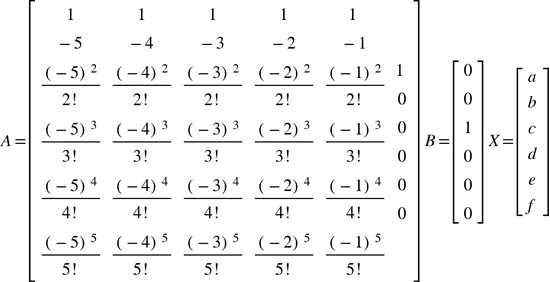
The weights are found with the help of MATLAB as follows:

A2=[1 1 1 1 1 1;
    -5 -4 -3 -2 -1 0;
    (-5)^2/f2 (-4)^2/f2 (-3)^2/f2 (-2)^2/f2 (-1)^2/f2 0;
    (-5)^3/f3 (-4)^3/f3 (-3)^3/f3 (-2)^3/f3 (-1)^3/f3 0;
    (-5)^4/f4 (-4)^4/f4 (-3)^4/f4 (-2)^4/f4 (-1)^4/f4 0;
    (-5)^5/f5 (-4)^5/f5 (-3)^5/f5 (-2)^5/f5 (-1)^5/f5 0];
b2=[0; 0; 1; 0; 0; 0];


X2=A2\b2
c2=[(-5)^6/f6 (-4)^6/f6 (-3)^6/f6 (-2)^6/f6 (-1)^6/f6 0]*X2

The above code was written as the continuation of the previous code. Hence the output will be in rational value which is shown as below

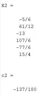
Hence the weights are

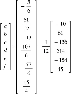
Here the output `c2` is the sum of coefficients in the column (7)

To prove that the order of approximation is fourth order, we can substitute the weights and find the sum of coefficients of `(7)`. It was found already from MATLAB output as `-137/180`.

We know sum of coefficients in `(1), (2), (4) ,(5)` and `(6)` are zero except `(3)` which is one.

So, expanding the Taylor's table we can get

`((Deltax)^2(d^2u)/dx^2)_(x=i) cong a.f(i-5)+b.f(i-4)+c.f(i-3)+d.f(i-2)+e.f(i-1) +f.f(i)=`

`0 + 0 + (Deltax)^2.f''(i) + 0 +0 + 0+(-137/180)(Deltax)^6.f^((vi))(i) + . . ."Higher order terms"`

Dividing throughout by `(Deltax)^2 ` we get

`((d^2u)/dx^2)_(x=i) cong ( a.f(i-5)+b.f(i-4)+c.f(i-3)+d.f(i-2)+e.f(i-1) +f.f(i))/(Deltax)^2`

`=0 + 0 + f''(i) + 0 +0 + (-137/180)(Deltax)^4.f^((vi))(i) + . . ."Higher order terms"`

So, it can be seen that the L.H.S will be our required approximation with the error of the order of `(Deltax)^4`

Now substituting the weights such as `a, b, c, d` and `e` in the equation `(V)` we get

`((d^2u)/dx^2)_(x=i) cong (45f(i)-154f(i-1)+214f(i-2)-156f(i-3)+61f(i-4) -10f(i-5))/(12(Deltax)^2)` ------ (Take it as)--`(VI)`

Step 3: Write the formula for different scheme as a function file in MATLAB

The formulae found from `(II),(IV) and (VI)` for Central differencing (CD) scheme, Skewed right sided differencing (SRD) scheme and Skewed left sided differencing(SLD) scheme respectively are fed in the function file as follows

function[sol_ana,sol_cdc,sol_sdr,sol_sdl]=discretization_2ndderivative_formula(x,dx)

f=@(x) exp(x).*cos(x); %Taking f(x) as a funciton
sol_ana=-2*exp(x).*sin(x); %formula for the analytical derivative

i=x; %position of x
i1=i+dx; %1st  node point forward
i2=i+2*dx;  %2nd  node point forward
i3=i+3*dx; %3rd  node point forward
i4=i+4*dx; %4th  node point forward
i5=i+5*dx; %4th  node point forward
i_1=i-dx; %1st  node point backward
i_2=i-2*dx; %2nd  node point backward
i_3=i-3*dx; %3rd  node point backward
i_4=i-4*dx; %3rd  node point backward
i_5=i-5*dx; %3rd  node point backward

sol_cdc=(-f(i_2)+16*f(i_1)-30*f(i)+16*f(i1)-f(i2))/(12*dx^2); % formula for central differencing scheme
sol_sdr=(45*f(i)-154*f(i1)+214*f(i2)-156*f(i3)+61*f(i4)-10*f(i5))/(12*dx^2); % formula for Skewed right handed differencing
sol_sdl=(45*f(i)-154*f(i_1)+214*f(i_2)-156*f(i_3)+61*f(i_4)-10*f(i_5))/(12*dx^2); % formula for Skewed left handed differencing

end

Step 4: Find the derivative for different values of `x` and `dx`

In order to understand the working of the formula for different point in space for the given function, we considered five values along the `x` axis arbitrarily as `x=[pi/40,pi/4,pi,pi/0.4,pi/0.04]`;

The space discretization was varied for each value of `x`. We can choose 50 equally spaced points between and alongwith `pi/4000` and `pi/4` for assigning different values of `dx`.

The code is attached below:

clear all
close all
clc

% Input x and dx values

x=[pi/40,pi/4,pi,pi/0.4,pi/0.04];
dx=linspace(pi/4000,pi/4,50) ;

% Call the function which handles the formula of discretization and find the..
% ..solution for different order of discretization
 for j=1:length(x)
    for i=1:length(dx)
   
[sol_ana(i,j),sol_cdc(i,j),sol_sdr(i,j),sol_sdl(i,j)]=discretization_2ndderivative_formula(x(j),dx(i));

err_cdc(i,j)=abs((sol_ana(i,j)-sol_cdc(i,j))); % Error for CDS
err_sdr(i,j)=abs((sol_ana(i,j)-sol_sdr(i,j)));% Error for Skewed Right sided
err_sdl(i,j)=abs((sol_ana(i,j)-sol_sdl(i,j)));% Error for Skewed Left sided
    end
end
% 
%Plot error in terms of different values of dx with the help of loglog plot
for j=1:length(x)
i=1:length(dx);
figure
loglog (dx,err_cdc(i,j),'s-', 'linewidth', 1.2)
hold on
loglog (dx,err_sdr(i,j),'s-','linewidth', 1.2)
loglog (dx,err_sdl(i,j),'s-','linewidth', 1.2)
legend({'Error for CDS','Error for Skewed Right sided','Error for Skewed Left sided'},'Location','northwest')
xlabel('dx')
ylabel('Error')
title(['Variation of Error at x = ',num2str(x(j),'%1.5f'),' for different values of "dx"'])

end

The ouput will be loglog plot for each value of `x` which shows the variation of Error for different values of `dx`. The outputs are attached and discussed as follows:

1)For `x=pi/40`

The output is shown below

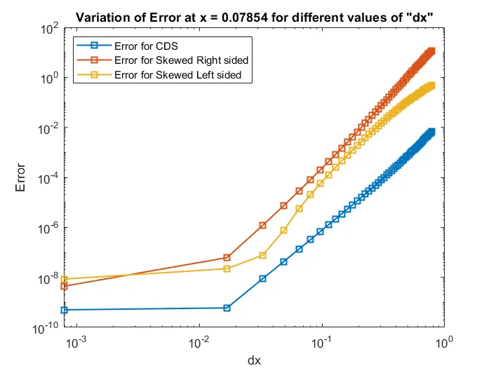
In this case, for all the values of `dx` error for CD scheme is lesser than the other two schemes. Also the error of SLD scheme is low compared to SRD scheme except when the value of `dx` is decreased below the order of `10^-2`. This may occur because of the round-off error.

2)For `x=pi/4`

The output is shown below

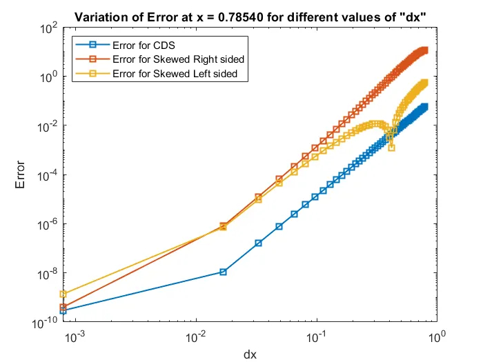
In this case also, for all the values of `dx` error for CD scheme is lesser than the other two schemes. Also the error of SLD scheme is low compared to SRD scheme except when the value of `dx` is decreased below the order of `10^-2` which is due to the round-off error.

3)For `x=pi`

The output is shown below

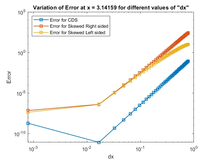
Error for CD scheme is lesser than the other two schemes here as well for all the values of `dx`. However the roundoff error caused the error value to increase when the value of `dx` is decreased below the order of `10^-2`. The error of SLD scheme is low compared to SRD scheme for all the values of `dx` that was considered. The slope of the error variation for all the schemes changed when the value of `dx` is decreased below the order of `10^-2`.

4)For `x=pi/0.4`

The output is shown below

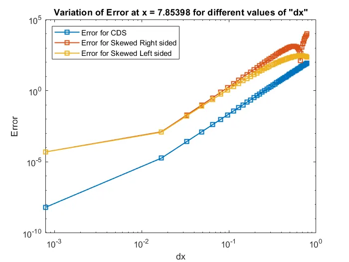
Error for CD scheme is lesser than the other two schemes for all the values of `dx`. Also, the error of SLD scheme is low compared to SRD scheme for all the values of `dx` that was considered except at the `dx` of 0.65. But still both the SRD and SLD schemes produce higher values of error at this point which is of the order of `10^4` which is not desirable. Also it can be noted that ,we can approach a value of error less than `10^-5` only with the CD scheme

5)For `x=pi/0.04`

The output is shown below

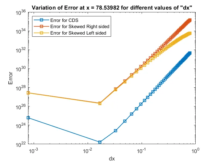
In this given case, eventhough the CD scheme had error less than the SRD and SLD schemes for all the values of `dx` it can be noted the errors are of order greater than `10^22`, which is not desirable.

Conclusion:

1) For all the values of `dx` considered, CD scheme produced less error compared to the skewed differencing schemes

2) When there is decrease of order of `dx` to less than `10^-2`, round off error comes into picture which changes the slope of the error variation for all the schemes

3) For the first four values values of `x` that was considered, CDS scheme produced a minimum error of less than `10^-6`. However for the highest value of `x` at `pi/0.04` , the error values are found to be of the order of greater than `10^22` which was undesirable.

4) All the schemes produced undesirable results when the value of `x` was `pi/0.04` for the considered values of 'dx'

Why Skewed scheme are preferred compared to CD scheme?

In some problems we may know the value of the function at one or the other sides of a node of interest. In this case CD scheme may not be applied since it requires information from both the sides of the nodes. At these conditions skewed differencing schemes are preferred compared to the CD scheme.