Week 5.1 - Mid term project - Solving the steady and unsteady 2D heat conduction problem

SOLVING THE STEADY AND UNSTEADY 2D HEAT CONDUCTION PROBLEM FOR THE GIVEN DOMAIN CONDITION:

OBJECTIVE: To solve the 2D heat conduction equation numerically for the given boundary condition, considering both steady state and unsteady state approach.

METHODOLOGY:

We assume the domain to be a square domain with 1 m length in both `x` and `y` axis as shown in figure below:

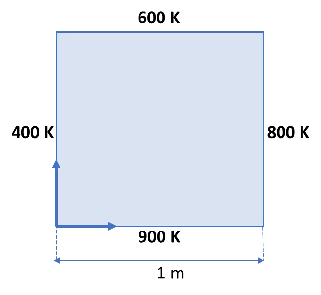
We will divide the domain into 10 nodes each in `x` and `y` directions. So there will be totally 100 nodes.

(i) Steady state analysis:

In the steady state analysis, the initial transient heating is omitted and the entire domain is assumed to have attained a temperature equilibrium. So the temperature at any point in the space within the given domain do not vary with time.

The steady state heat transfer equation is given by:

`(del^2T)/(delx^2)+(del^2T)/(dely^2)=0`

Now we consider any node and name it as `P` in the domain. We discretise the above equation on the particular node as follows:

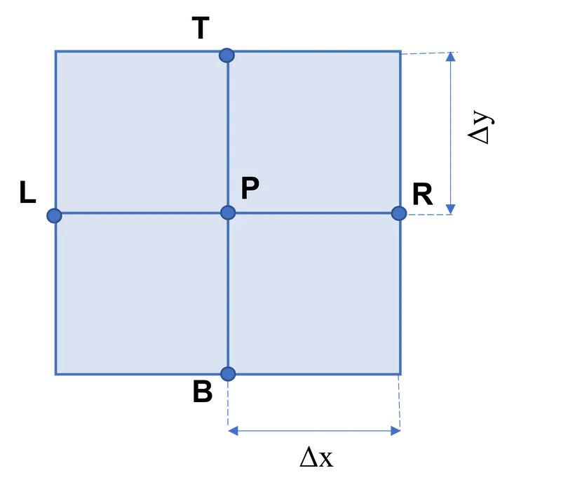
`(T_L-2T_P+T_R)/((Deltax)^2)+(T_T-2T_P+T_B)/((Deltay)^2)=0`

Now separating the `T_P` component we get,

`T_P=(1/k)((T_L+T_R)/((Deltax)^2)+(T_T+T_B)/((Deltay)^2))` --------------(I)

where `k=(2((Deltax)^2+(Deltay)^2))/((Deltax)^2(Deltay)^2)`

Now we will find the solution at each node point by iterative methods such as (1) Gauss Jacobi, (2) Gauss Siedel and (3) Successive overrelaxation method.

(ii) Unsteady state analysis:

In the unsteady state analysis, there is a transient heating initially and if the temperature at the boundaries are kept constant, the temperature inside the domain attains an equllibrium condition after certain time. Now in this analysis we will find how the Temperature is varying in the initial transient heating stage and how much time is needed to attain the steady state equillibrium.

The unsteady state heat transfer equation is given by:

`(del^2T)/(delx^2)+(del^2T)/(dely^2)=1/alpha.(delT)/(delt)`

where `alpha` is the thermal diffusivity,

In our analysis, we will assume the thermal diffusivity value to be 1.4 `m^2`/s.

Now if we discretise the above equation (2) at a node `P` (in the same way as considered previously), we get

`(T_L-2T_P+T_R)/((Deltax)^2)+(T_T-2T_P+T_B)/((Deltay)^2)=(T_P^(n+1)-T_p^n)/(Deltat)`

where the superscript `n` denotes the Temperature value of the corresponding node at the '`n`'th time step.

Now if we rearrange the above equation, we get,

`T_P^(n+1)=T_P^n+k_1*(T_L^(n or n+1)-2T_P^(n or n+1)+T_R^(n or n+1))+k_2*(T_T^(n or n+1)-2T_P^(n or n+1)+T_B^(n or n+1))` ------------- (II)

where `k_1=alpha.(Deltat)/(Deltax)^2` and `k_2=alpha.(Deltat)/(Deltay)^2`

and the second and third terms in the RHS may contain the temperature values either of the `n` th time step or the `n+1` th time step.

If we take it as `n` th time step, we know the temperature value of all the node points explicitly and we call it as Explicit method. And if we take the Temperature values at `n+1` th time step we may not know the values of all the corresponding nodes and we may need to find the solution with help of some iterative techniques. We call this method as Implicit method.

So in order to solve the Unsteady state heat transfer equation, we may either choose Explicit scheme or Implicit Scheme. In our present problem we analyse the solution with the help of 1) Explicit method 2) Implicit method-with Gauss Jacobi scheme 3) Implicit method with Gauss Seidel scheme and 4) Implicit method with Successive overrelaxation scheme.

SOLUTION:

(1)STEADY STATE ANALYSIS

Now we will solve the steady state equation based on the discretisation formula (I) derived previously with each of the following iterative schemes

(1)-(i) Gauss Jacobi Scheme:

Let `i` denotes the `i` th row and `j` denotes the `j`th column. Then `T_(i,j)` denotes the Temperature at the node placed at `i` th row and `j` th column. Now we will rewrite the discretisation formula based on the indices considered as follows:

`T_(i,j)^(q+1)=(1/k)((T_(i-1,j)^(q)+T_(i+1,j)^(q))/((Deltax)^2)+(T_(i,j-1)^(q)+T_(i,j+1)^(q))/((Deltay)^2))`

where `k=(2((Deltax)^2+(Deltay)^2))/((Deltax)^2(Deltay)^2)` and superscript `q` denotes `q` th iteration

In Gauss Jacobi scheme, we find the value of the given node, say `T_(i,j)` at `q+1` th iteration by considering the previous iteration values (`q` th iteration) of the neighbouring nodes.

After that we solve the above formula for each node and find the solution by iteration until `T_(i,j)^(q+1)-T_(i,j)^q<=1e^-4`

(1)-(ii) Gauss Siedel Scheme:

In Gauss Siedel scheme, we find the value of the given node, say `T_(i,j)` at `q+1` th iteration by considering the known values of neighbouring nodes from `q+1` th iteration and unknown neighbouring values from the previous iteration(`q` th iteration).

The discretisation formula can be given as:

`{T_(i,j)^(q+1)}_(GS)=(1/k)((T_(i-1,j)^(q+1)+T_(i+1,j)^(q))/((Deltax)^2)+(T_(i,j-1)^(q+1)+T_(i,j+1)^(q))/((Deltay)^2))`

After that we iterate until the required tolerance `1e^-4` is achieved.

(1)-(iii) Successive Over Relaxation(SOR) Scheme:

In successive overrelaxation scheme, we extrapolate the Gauss seidel method for faster convergence by considering the weighted average of the previous iteration value and the Gauss seidel iteration value of the current iteration.

The discretisation formula is given by:

`{T_(i,j)^(q+1)}_(SOR)=(1-omega)*T_(i,j)^(q)+omega*{T_(i,j)^(q+1)}_(GS)`

We iterate the solution as the same way, until the required tolerance of `1e^-4` is achieved.

Matlab code for steady state solver:

All the above three schemes will be solved with the help of a MATLAB code which is attached below:

%2D Heat conduction solver steady state
clear 
close all
clc

%Forming the domain
nx=10; %number of 'x' nodes
ny=10; %number of 'y' nodes
x=0:1/(nx-1):1; %Coordinates of x
y=0:1/(ny-1):1; %Coordinates of y
delx=1/(nx-1); %spatial discretisation along x
dely=1/(ny-1); %spatial discretisation along y

%Initial Temperature distribution
u=300*ones(10);
u(1,1:ny)=900; %Bottom nodes
u(1:nx,1)=400; %Left nodes
u(nx,1:ny)=600; %Top nodes
u(1:nx,ny)=800; %Right nodes
%Taking average temperature at the corner points
u(1,1)=0.5*(u(1,2)+u(2,1)); 
u(1,ny)=0.5*(u(1,ny-1)+u(2,ny));
u(nx,1)=0.5*(u(nx-1,1)+u(nx,2));
u(nx,ny)=0.5*(u(nx-1,ny)+u(nx,ny-1));
uold=u;
uinitial=u;

prompt = 'Choose an iterative scheme nEnter 1 for GAUSS JACOBI nEnter 2 for GAUSS SIEDEL nEnter 3 for SUCCESSIVE OVER RELAXATIONn';
Iterative_solver= input(prompt);

%Solution Gauss Jacobi
if Iterative_solver==1
k=2*(delx^2+dely^2)/(delx^2*dely^2);
jacobi_iter=1;
tol=1;
while tol>1e-4
for i=2:nx-1
    for j=2:ny-1
        term1=(1/k)*(uold(i-1,j)+uold(i+1,j))/delx^2;
        term2=(1/k)*(uold(i,j-1)+uold(i,j+1))/dely^2;
        u(i,j)=(term1+term2);
    end
end
tol=(max(max(abs(uold-u))));
uold=u;
jacobi_iter=jacobi_iter+1;
contourf(x,y,u,'--','ShowText','on');
colormap(jet);
colorbar;
text=sprintf('Iteration number = %d',jacobi_iter);
title('TEMPERATURE PLOT - GAUSS JACOBI', text)
xlabel('X-axis')
ylabel('Y-axis')
pause(0.03)
end
fprintf('Iteration ended after %d times with a maximum error of %e for Gauss Jacobi methodn',jacobi_iter,tol)

%Solution Gauss siedel
elseif Iterative_solver==2
k=2*(delx^2+dely^2)/(delx^2*dely^2);
gs_iter=1;
tol=1;
while tol>1e-4
for i=2:nx-1
    for j=2:ny-1
        term1=(1/k)*(u(i-1,j)+uold(i+1,j))/delx^2;
        term2=(1/k)*(u(i,j-1)+uold(i,j+1))/dely^2;
        u(i,j)=(term1+term2);
    end
end
tol=(max(max(abs(uold-u))));
uold=u;
gs_iter=gs_iter+1;
contourf(x,y,u,'--','ShowText','on');
colormap(jet);
colorbar;
text=sprintf('Iteration number = %d',gs_iter);
title('TEMPERATURE PLOT - GAUSS SIEDEL', text)
xlabel('X-axis')
ylabel('Y-axis')
pause(0.03)
end
fprintf('Iteration ended after %d times with a maximum error of %e for Gauss Siedel methodn',gs_iter,tol)

%Solution Successive over relaxation
elseif Iterative_solver==3
k=2*(delx^2+dely^2)/(delx^2*dely^2);
ii=1;
for w=[-0.2,0.2,0.6,1.0,1.4,1.8,2.2] %Relaxation factor
sor_iter=1;
tol=1;
ugs=uinitial;
uold=uinitial;
u=uinitial;
while tol>1e-4
for i=2:nx-1
    for j=2:ny-1
        term1=(1/k)*(u(i-1,j)+uold(i+1,j))/delx^2;
        term2=(1/k)*(u(i,j-1)+uold(i,j+1))/dely^2;
        ugs(i,j)=(term1+term2);
        u(i,j)=(1-w)*uold(i,j)+w*ugs(i,j);
    end
end
tol=(max(max(abs(uold-u))));
uold=u;
sor_iter=sor_iter+1;
if sor_iter>2000
    fprintf('The solution is diverging for relaxation factor = %0.1f;n',w)
    break
end
end
figure;
contourf(x,y,u,'--','ShowText','on');
colormap(jet);
colorbar;
text=sprintf('Iteration number = %d, Relaxation factor = %0.1f',sor_iter,w);
title('TEMPERATURE PLOT - SUCCESSIVE OVERRELAXATION METHOD', text)
xlabel('X-axis')
ylabel('Y-axis')
fprintf('Iteration ended after %d times with a maximum error of %e for Successive overrelaxation methodn for relaxation factor = %.1fn',sor_iter,tol,w)
SOR_ITER(ii)=sor_iter;
w1(ii)=w;
ii=ii+1;
end
figure;
b=bar(w1,SOR_ITER,'FaceColor','flat');
xlabel('Relaxation factor')
ylabel('Number of iterations')
title('SUCCESSIVE OVERRELAXATION METHOD','Study of Relaxation Factor on Number of iterations')
xtips1 = b.XEndPoints;
ytips1 = b.YEndPoints;
labels1 = string(b.YData);
clear text
text(xtips1,ytips1,labels1,'HorizontalAlignment','center','VerticalAlignment','bottom')
b.CData(1,:) =[0.8 0 0];b.CData(7,:)=[0.8 0 0];b.CData(5,:)=[0 0.8 0]; %Colour of the bar altered after studying the result.

elseif Iterative_solver~=1||2||3
    fprintf('Error:Choice should be either of 1,2 or 3')
end

1-(iv):Results of Steady state analysis

The programme was written in an interactable format and the user might need to specify which method to be used for executing the programme. Based on the selection the programe will execute the output.

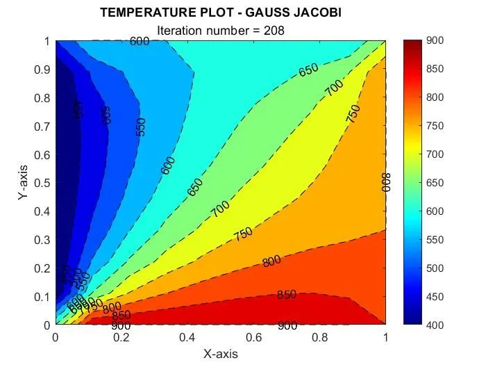
Gauss Jacobi Scheme:

The iteration ended after 208 times and the final Temperature profile is shown below:

The MATLAB output is attached below:

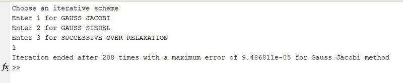
The maximum error was `9.486811"x"10^-5` between the final result and previous iteration.

Gauss Siedel Scheme:

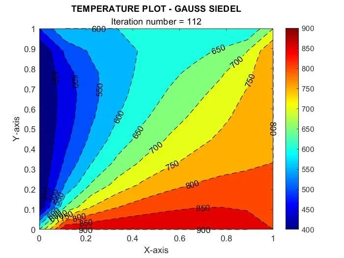
The same temperature profile was obtained for the Gauss siedel scheme. But the solution was obtained after 112 iterations itself. The final Temperature profile is shown below:

The MATLAB output is attached below:

Successive Over-Relaxation(SOR) scheme:

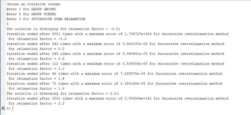
From various references, it was found that relaxation factor should be between 0 and 2 for convergence. Hence, in our current study seven values were considered as `omega=[-0.2,0.2,0.6,1.0,1.4,1.8,2.2]`. The same temperature profile as in previous two schemes was obtained for the SOR scheme. But the solution was obtained after different number of iterations for different relaxation factor.

The MATLAB output is attached below:

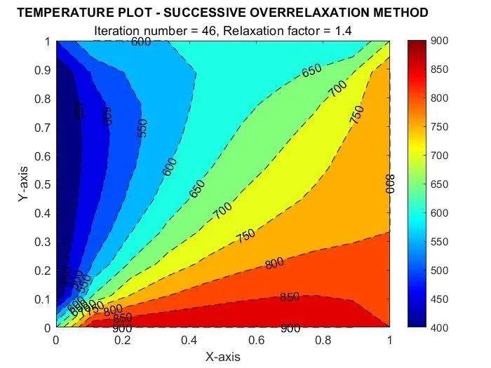
The converged solution is attached below for the relaxation factor of `omega=1.4`:

The solution is diverged for the relaxation factor of `omega=-0.2` and `omega=2.2`. The program was stopped after a maximum of 2001 iteration and the diverged result is shown below for the relaxation factor of `omega=2.2`:

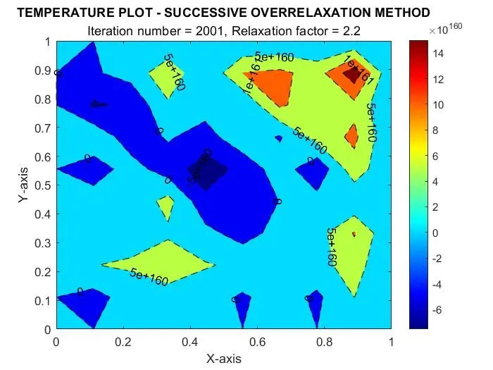
It was observed that for the relaxation factor between `0` and `2` the solution converged and for the remaining values that were considered the solution was found to be diverging. The comparison is shown below:

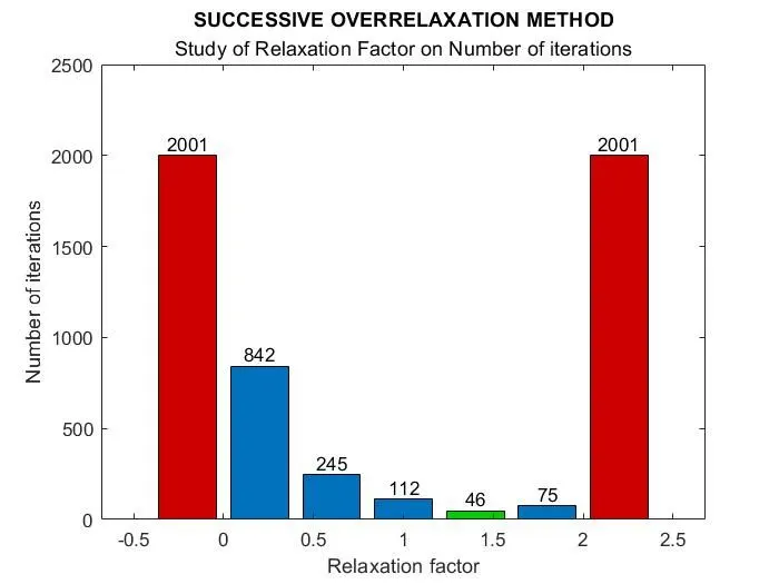
It can be noted that the solution converged at a minimum number of iterations when `omega=1.4` (among the studied values). It can also be seen that the solution converged after 112 times for `omega=1` which is equivalent to the number of iterations of the Gauss siedel scheme. Because `omega=1` the SOR scheme becomes the Gauss siedel scheme itself as per the formula.

(2)UNSTEADY STATE ANALYSIS

Now we will solve the unsteady state equation based on the discretisation formula (II) derived previously with each of the following schemes:

(2)-(i) Explicit Scheme:

In Explicit scheme, at each time step the discretisation formula was solved for the values which are known at the previous time step.

The discretisation formula is given by:

`T_(i,j)^(n+1)=T_(i,j)^n+k_1*(T_(i-1,j)^(n)-2T_(i,j)^(n)+T_(i+1,j)^(n))+k_2*(T_((i,j-1))^n-2T_(i,j)^(n)+T_(i,j+1)^(n))`

Where `k_1=alpha.(Deltat)/(Deltax)^2` and `k_2=alpha.(Deltat)/(Deltay)^2`

Rearranging we get,

`T_(i,j)^(n+1)=(1-2k_1-2k_2)T_(i,j)^n+k_1*(T_(i-1,j)^(n)+T_(i+1,j)^(n))+k_2*(T_(i,j-1)^(n)+T_(i,j+1)^(n))`

The above formula is solved until the equilibrium temperature is attained. The Temperature was said to be steady if the maximum difference at a nodal temperature between the current time step and the previous time step was less than or equal to `1"x"10^-4`

(2)-(ii) Implicit-Gauss Jacobi Scheme:

In Implicit-Gauss Jacobi scheme, at each time step the discretisation formula was iterated until the tolerance is achieved with the help of the previous iteration values of the neighbouring nodes from the current time step itself.

The discretisation formula is given by:

`T_(i,j)^(n+1)=T_(i,j)^n+k_1*(T_(i-1,j)^(n+1)-2T_(i,j)^(n+1)+T_(i+1,j)^(n+1))+k_2*(T_(i,j-1)^(n+1)-2T_(i,j)^(n+1)+T_(i,j+1)^(n+1))`

Where `k_1=alpha.(Deltat)/(Deltax)^2` and `k_2=alpha.(Deltat)/(Deltay)^2`

Rearranging and including superscript `q` for iteration number we can write,

`T_(i,j)^(n+1,q+1)=1/(1+2k_1+2k_2)(T_(i,j)^n+k_1*(T_(i-1,j)^(n+1,q)+T_(i+1,j)^(n+1,q))+k_2*(T_(i,j-1)^(n+1,q)+T_(i,j+1)^(n+1,q)))`

Here the tolerance is given by `T_(i,j)^(n+1,q+1)-T_(i,j)^(n+1,q)`. If the tolerance is less than `10^-4`, the temperature value at `q+1` th iteration is taken as the solution at that particular time step. Then the time step is increased and the iteration procedure is repeated for the solution at the next time step. This procedure is repeated until `T_(i,j)^(n+1)-T_(i,j)^(n)<=10^-4` , i.e.,steady state is achieved.

(2)-(iii) Implicit-Gauss Siedel Scheme:

In Implicit-Gauss Siedel scheme, at each time step the discretisation formula was iterated until the tolerance is achieved with the help of the unknown previous iteration values and the known current iteration values as well(which are known) from the current time step itself.

The discretisation formula can be written as:

`{T_(i,j)^(n+1,q+1)}_(GS)=1/(1+2k_1+2k_2)(T_(i,j)^n+k_1*(T_(i-1,j)^(n+1,q+1)+T_(i+1,j)^(n+1,q))+k_2*(T_(i,j-1)^(n+1,q+1)+T_(i,j+1)^(n+1,q)))`

Where `k_1=alpha.(Deltat)/(Deltax)^2` and `k_2=alpha.(Deltat)/(Deltay)^2`

Same iterative procedure which was discussed as in Gauss Jacobi scheme was used.

(2)-(iv) Implicit-Successive Over Relaxation (SOR) Scheme:

In Implicit-SOR scheme,we extrapolate the Gauss seidel method for faster convergence by considering the weighted average of the previous iteration value and the Gauss seidel iteration value of the current iteration.

The discretisation formula is given by:

`{T_(i,j)^(n+1,q+1)}_(SOR)=(1-omega)*T_(i,j)^(n+1,q)+omega*{T_(i,j)^(n+1,q+1)}_(GS)`

Here the relaxation factor was assumed as `omega=1.4`. Because from our previous experience, we obtained a minimum number of iteration for the relaxation factor of `1.4` for the steady state-successive over relaxation scheme.

Achieving stability criteria:

Courant number is given by `CFL=CFL_x+CFL_y` where `CFL_x=alpha.(Deltat)/(Deltax)^2 " and " CFL_y=alpha.(Deltat)/(Deltay)^2`

For all the schemes, we assume that the courant number to be 0.25(that is `CFL_x=CFL_y=0.25`). Because as per the stability criteria, for explicit scheme the courant number should be less than 0.5(i.e., `CFL=CFL_x+CFL_y<=0.5`) . Though the implicit scheme is unconditionally stable, the courant number is assumed to be 0.25 uniformly for all the schemes.

Matlab code for unsteady state solver:

All the above four schemes will be solved with help of the MATLAB code which is attached below:

%2D Heat conduction-Transient solver 
clear 
close all
clc

%Forming the domain
nx=10; %number of 'x' nodes
ny=10; %number of 'y' nodes
x=0:1/(nx-1):1; %Coordinates of x
y=0:1/(ny-1):1; %Coordinates of y
delx=1/(nx-1); %spatial discretisation along x
dely=1/(ny-1); %spatial discretisation along y
alpha=1.4; %Thermal diffusivity
cfl=0.25; %Taking CFL_x or CFL_y =0.2
delt=cfl*delx^2/alpha; %or delt=cfl*dely^2/alpha

%Initial Temperature distribution
u=300*ones(10);
u(1,1:ny)=900; %Bottom nodes
u(1:nx,1)=400; %Left nodes
u(nx,1:ny)=600; %Top nodes
u(1:nx,ny)=800; %Right nodes
%Taking average temperature at the corner points
u(1,1)=0.5*(u(1,2)+u(2,1)); 
u(1,ny)=0.5*(u(1,ny-1)+u(2,ny));
u(nx,1)=0.5*(u(nx-1,1)+u(nx,2));
u(nx,ny)=0.5*(u(nx-1,ny)+u(nx,ny-1));
uold=u;
uinitial=u;

prompt = 'Choose an iterative scheme n1 FOR EXPLICIT n2 FOR IMPLICIT-GAUSS JACOBI n3 FOR IMPLICIT-GAUSS SEIDEL n4 FOR IMPLICIT-SUCCESSIVE OVER RELAXATIONn';
Iterative_solver= input(prompt);

%Solution Explicit Scheme
if Iterative_solver==1
k1=alpha*delt/delx^2;
k2=alpha*delt/dely^2;
for nt=1:10000
for i=2:nx-1
    for j=2:ny-1
        term1=k1*(uinitial(i-1,j)+uinitial(i+1,j));
        term2=k2*(uinitial(i,j-1)+uinitial(i,j+1));
        u(i,j)=(1-2*k1-2*k2)*uinitial(i,j)+term1+term2;
    end
end
steady=max(max(abs(uinitial-u)));

if steady<1e-4
    break
end
contourf(x,y,u,'--', 'ShowText','on');
colormap(jet);
colorbar;
text=sprintf('Time = %0.4f seconds',nt*delt);
title('TEMPERATURE PLOT - EXPLICIT SCHEME', text)
xlabel('X-axis')
ylabel('Y-axis')
pause(0.003)
uinitial=u;
end
fprintf('The steady state was achieved after %0.4f seconds for Explicit scheme with an error of %d',(nt-1)*delt,steady)

%Solution Implicit-Gauss Jacobi
elseif Iterative_solver==2
k1=alpha*delt/delx^2;
k2=alpha*delt/dely^2;
for nt=1:10000
for iter=1:10000
for i=2:nx-1
    for j=2:ny-1
        term1=k1*(uinitial(i-1,j)+uinitial(i+1,j));
        term2=k2*(uinitial(i,j-1)+uinitial(i,j+1));
        u(i,j)=1/(1+2*k1+2*k2)*(uold(i,j)+term1+term2);
    end
end
tol=(max(max(abs(uinitial-u))));
uinitial=u;
if tol<1e-4
    break
end
end
steady=max(max(abs(uold-u)));
if steady<1e-4
    break
end
uold=u;
contourf(x,y,u,'--', 'ShowText','on');
colormap(jet);
colorbar;
text=sprintf('Time = %0.4f seconds',nt*delt);
title('TEMPERATURE PLOT - IMPLICIT - GAUSS JACOBI', text)
xlabel('X-axis')
ylabel('Y-axis')
pause(0.003)
end
fprintf('The steady state was achieved after %0.4f seconds for Implicit-Gauss Jacobi scheme with an error of %d',(nt-1)*delt,steady)

%Solution Implicit-Gauss Siedel
elseif Iterative_solver==3
k1=alpha*delt/delx^2;
k2=alpha*delt/dely^2;
for nt=1:10000
for iter=1:10000
for i=2:nx-1
    for j=2:ny-1
        term1=k1*(u(i-1,j)+uinitial(i+1,j));
        term2=k2*(u(i,j-1)+uinitial(i,j+1));
        u(i,j)=1/(1+2*k1+2*k2)*(uold(i,j)+term1+term2);
    end
end
tol=(max(max(abs(uinitial-u))));
uinitial=u;
if tol<1e-4
    break
end
end
steady=max(max(abs(uold-u)));
if steady<1e-4
    break
end
uold=u;
contourf(x,y,u,'--', 'ShowText','on');
colormap(jet);
colorbar;
text=sprintf('Time = %0.4f seconds',nt*delt);
title('TEMPERATURE PLOT - IMPLICIT - GAUSS SEIDEL', text)
xlabel('X-axis')
ylabel('Y-axis')
pause(0.003)
end
fprintf('The steady state was achieved after %0.4f seconds for Implicit-Gauss Siedel scheme with an error of %d',(nt-1)*delt,steady)

%Solution Successive over relaxation
elseif Iterative_solver==4
k1=alpha*delt/delx^2;
k2=alpha*delt/dely^2;
ugs=u;
w=1.4; %Relaxation factor
for nt=1:10000
for iter=1:100000
for i=2:nx-1
    for j=2:ny-1
        term1=k1*(u(i-1,j)+uinitial(i+1,j));
        term2=k2*(u(i,j-1)+uinitial(i,j+1));
        ugs(i,j)=1/(1+2*k1+2*k2)*(uold(i,j)+term1+term2);
        u(i,j)=(1-w)*uinitial(i,j)+w*ugs(i,j);
    end
end
tol=(max(max(abs(uinitial-u))));
uinitial=u;
if tol<1e-4
    break
end
end
steady=max(max(abs(uold-u)));
if steady<1e-4
    break
end
uold=u;
contourf(x,y,u,'--', 'ShowText','on');
colormap(jet);
colorbar;
text=sprintf('Time = %0.4f seconds, Relaxation factor = %0.1f',nt*delt,w);
title('TEMPERATURE PLOT - IMPLICIT - SUCCESSIVE OVERRELAXATION', text)
xlabel('X-axis')
ylabel('Y-axis')
pause(0.003)
end
fprintf('The steady state was achieved at %0.4f seconds for Implicit-Successive over relaxation scheme with an error of %dnThe Relaxation factor was %0.1f',(nt-1)*delt,steady,w)

elseif Iterative_solver~=1||2||3||4
    fprintf('Error:Choice should be either of 1,2,3 or 4')
end

(2)-(v) Results of the Unsteady state solver:

For each of the above schemes discussed, the final temperature profile, time to achieve the steady state and the tolerance was noted. The results are discussed below:

Explicit Scheme:

The temperature profile and the MATLAB output is attached below:

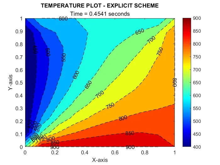
The steady state i.e., temperature distribution attained an equilibrium state after 0.4541 seconds. The temperature profile was found to be similar to that of the solution obtained with help of the steady state solver.

Implicit-Gauss Jacobi Scheme:

The temperature profile and the MATLAB output is attached below:

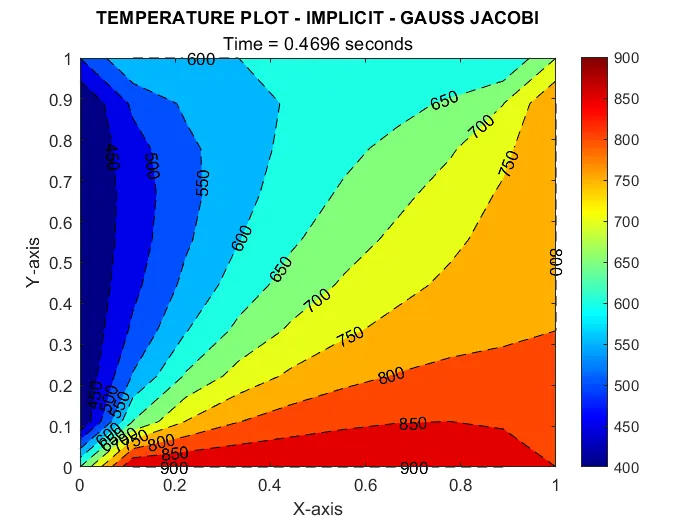
A similar temperature profile was obtained. The equilibrium temperature was obtained after 0.4696 seconds. The difference between the time may be due to the numerical diffusion since we used the iterative technique in the implicit scheme.

Implicit-Gauss Siedel Scheme:

The temperature profile and the MATLAB output is attached below:

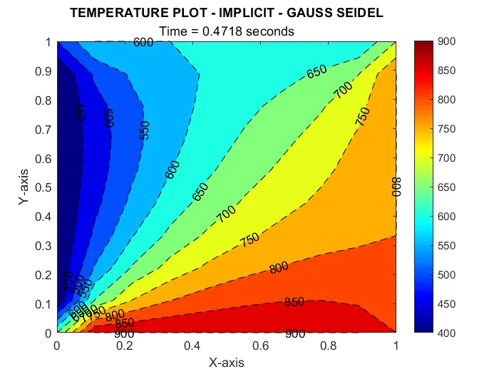
The temperature equilibrium was obtained at a time of 0.4718 seconds which was almost similar to the Implicit Gauss Jacobi scheme.

Implicit-SOR Scheme:

The relaxation factor was assumed to be 1.4 as discussed previously. The temperature profile and the MATLAB output is attached below:

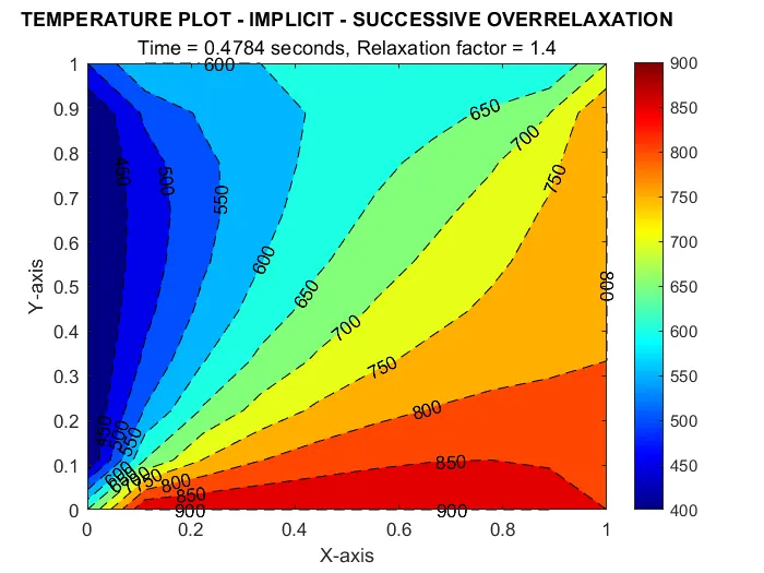
The temperature profile obtained was correct as predicted by the previous other schemes. The difference in time for attaining the steady state temperature may be due the numerical diffusion.

CONCLUSION:

The steady and unsteady state solver for a given problem considering the given domain was solved numerically.

1) All the solvers produced an identical temperature profile with the given tolerance.

2) For the steady state heat conduction equation, three different iterative solvers were compared. It was found that the SOR scheme produced the required solution at the minimum number of iterations for a relaxation factor of 1.4. It was also found that solution diverged when the relaxation factor value was not between 0 and 2 for the SOR scheme.

3) For the unsteady state heat conduction equation, explicit scheme and implicit scheme (with three different iterative solvers) were compared. Though implicit scheme is unconditionally stable the time to attain the steady state temperature was found to be different from the explicit scheme. This may be due to the numerical diffusion because of the iterative schemes utilised in the implicit method.