Week 7 - Simulation of a 1D Super-sonic nozzle flow simulation using Macormack Method
Aim: To simulate an isentropic flow through a quasi 1-D subsonic - supersonic nozzel and derive both conservative and non-conservative form of governing equations and solve them using MacCormak's tecnique.
Also to plot the following
1. Steady-state distribution of primitive variables inside the nozzle
2. Time-wise variation of the primitive variables
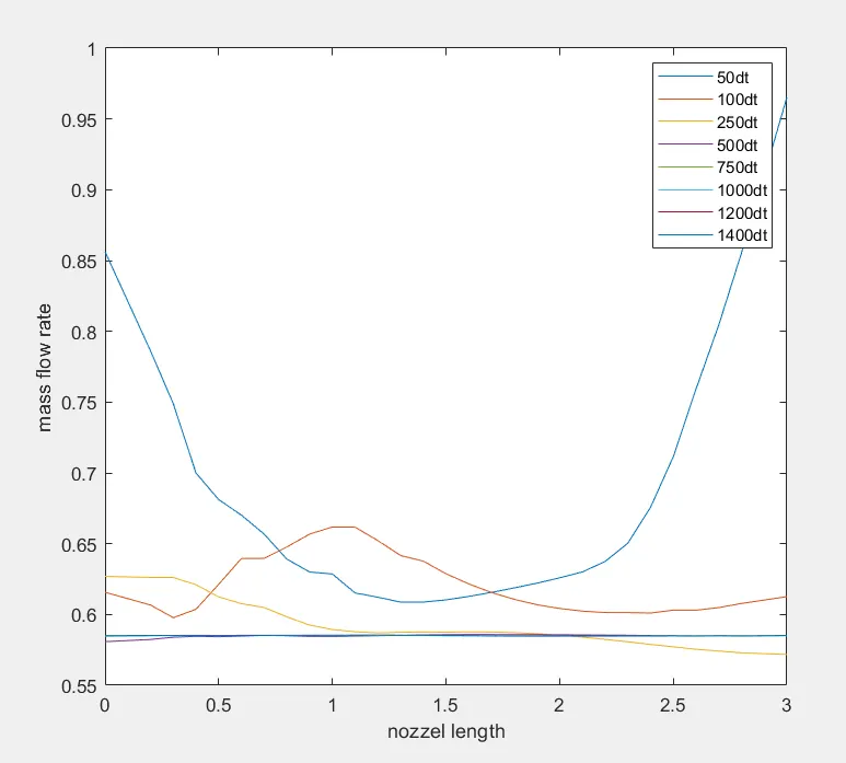
3. Variation of Mass flow rate distribution inside the nozzle at different time steps during the time-marching process
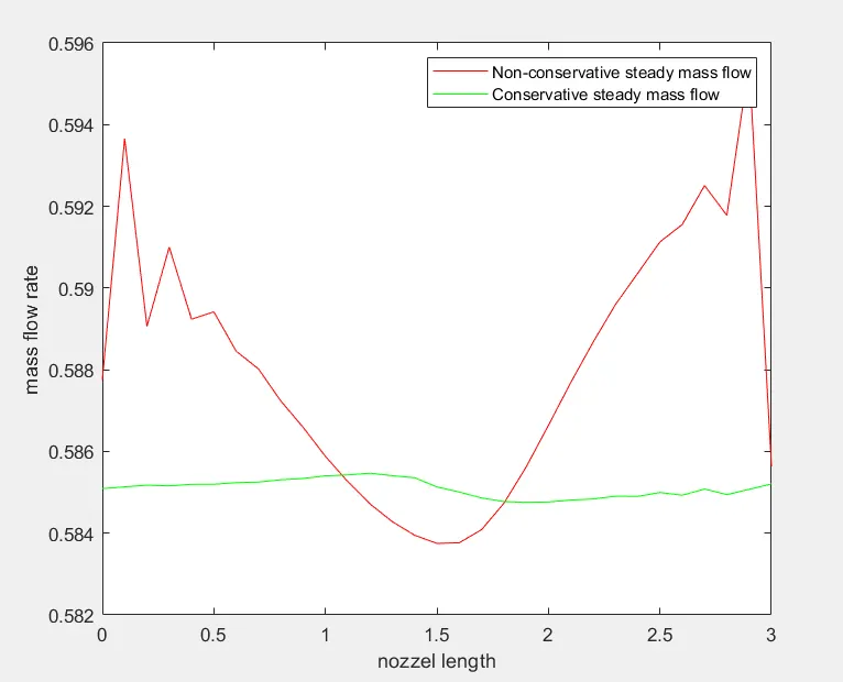
4. Comparison of Normalized mass flow rate distributions of both forms
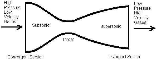
Theory: Nozzel is a device with variable crosssectional area designed to control the direction and flowrate of fluid through it as it exits and enclosed chamber or pipe.Specifically it is used to increase or decrease the velocity and hence other properties.There are different types of nozzels and here in our project we will be using a Convergernt-Divergent nozzzel. The convergent section of the nozzel has a fluid in subsonic state(i.e.Ma<1) and as the fluid exits the divergent part it is in supersonic state (i.e.Ma>1).The figure below shows our nozzel.
Here we assume that the flow at the inlet is from a reservoirwhere pressure and temperature are denoted by `P_o`and `T_o` . The crossesctional area at reservoir is very large(`a= infty`) and henve velocity(v) is zero(0).Thus `P_0` and `T_o` are Stagnation Pressure and Stagnation Temperature.The flow expands isentropically at the exit where exit Pressure,Temperature,density,mach number are denoted as `P_e,T_e,rho_e,M_e`.The flow is sonic at throat i.e velocity of flow is equal to velocity of sound in that fluid at throat.
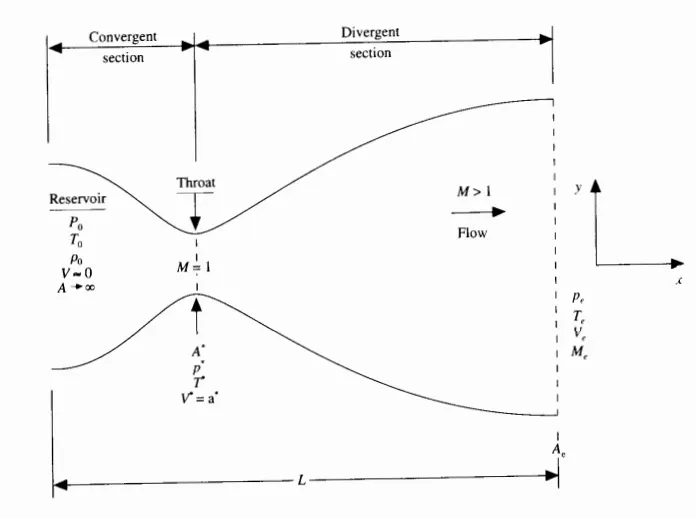
We assume that the flow properties are uniform at a section and hence it varies only along the length of the nozzel and our problem becomes a quasi 1-D flow problem.
Steps to solve the probelm:
1) governing equations in both Conservation and Non conservation form
2) finite differencing pertaining to MAcCormack's technique
Governing equations in Non-Conservation form:
*Continuity: `(delrho')/(delt')= -rho'*(delV')/(delx') -rho'*V'*(del(logA'))/(delx') - V'*(delrho')/(delx')`
*Momentum: `(delV')/(delt')= -V'*(delV')/(delx') -1/gamma *( (delT')/(delx')+ (T')/rho' *(delrho')/(delx'))`
*Energy: `(delT')/(delt')=-V'*(delT')/(delx') -(gamma-1)*T'*[(delV')/(delx') + V'*(del(log(A')))/(delx')]`
All variables are in non dimensional forms
Initial condtions for Non Conservative form are
`rho=1-0.3146x`
`t=1-0.2314x`
`A=1+2.2(x-1.5)^2`
Governing equations in Conservative form:
*Continuity: `(delrho'A')/(delt')=-(delrho'A'V')/(delx')`
*Momentum:`(delrho'A'V')/(dt')+ (del(rho'A'V'^2)+(1/gamma)*A'V')/(delx')=(1/gamma*rho'*(delA')/(delx')`
*Energy: `(del(rho'*(T'*1/(gamma-1) +(gamma/2)*V'^2)*A'))/(delt')= (del(rho'*(T'*1/(gamma-1) +(gamma/2)*V'^2)*A'+ rho'*A'*V'))/(delx')`
The above equations can be further simplified in terms of Flux vectors ,solution Vectors and source term as follows.
`(delU_1)/(delt')=- (delF_1)/(delx')`
`(delU_2)/(delt') =-(delF_2)/(delx') +J_2`
`(delU_3)/(delt')=-(delF_3)/(delx')`
where `U_1=rho'.A'`
`U_2=rho'*A'*V'`
`U_3=rho'*(T'*1/(gamma-1) +(gamma/2)*V'^2)*A'`
`F_1=rho'*A'*V'`
`F_2= rho'*A'*V'^2 + 1/gamma *rho'*A'`
`F_3=rho'*(T'*1/(gamma-1) +(gamma/2)*V'^2)*A'*V' +rho'*A'*V'`
`J_2=1/gamma *rho'(delA')/(delx')`
Here `U_1,U_2,U_3` are called the solution vectors, `F_1,F_2,F_3` are called the Flux terms and `J_2`is the source term.
MacCormack's Method:
In MacCormack's method we address a time marching solution assuminf flow at each grid point at time t to be know inorder to find flow varibales at `t + Deltat`.It is a predictor-corrector approach.Firstly we go with the predictor step.All the spatial derivatives are done with forward differencing.So we will have
For Non-Conservative form:
`((delrho)/(delt))_(ip)^t= -rho_i^t*(V_(i+1)^t -V_i^t )/(Deltax) -rho_i^t*V_i^t*(lnA_i+1 -lnA_i)/(Deltax) -V_i^t*(rho_(i+1)^t -rho_i^t )/(Deltax)`
`((delV)/(delt))_(ip) ^t = -V_i^t*(V_(i+1)^t -V_i^t)/(Deltax) -(1/gamma)*(((T_i+1^t -T_i^t)/(Deltax))+T_i^t /rho_i^t *(rho_(i+1) ^t -rho_i^t)/(Deltax))`
`((delT)/(delt))_(ip)^t=-V_i^t*(T_(i+1)^t -T_i^t)/(Deltax) -(gamma-1)*T_i^t*((V_(i+1)^t -V_i^t)/(Deltax) +V_i^t*(lnA_(i+1) -lnA_i)/(Deltax))`
By usuing the above forward differencing approach we get the predicted value of our primitive varibales as foloows:
`rho_(ip)^(t+Deltat) =rho_i^t +((delrho)/(delt))_(ip)^t*Deltat`
`v_(ip)^(t+Deltat) =v_i^t +((delv)/(delt))_(ip)^t*Deltat`
`T_(ip)^(t+Deltat) =T_i^t +((delT)/(delt))_(ip)^t*Deltat`
We got the values for `rho_i,T_i,V_i` at time t.Now moving to the corrector step we replace the forward differencing with rearward differencing and find the value of `(delrho)/(delt) ,(delV)/(delt),(delT)/(delt)` as follows:
`((delrho)/(delt))_(ic)^(t+Deltat)= -rho_i^t*(V_(i)^t -V_(i-1) ^t )/(Deltax) -rho_i^t*V_i^t*(lnA_i -lnA_(i-1))/(Deltax) -V_i^t*(rho_(i)^t -rho_(i-1)^t )/(Deltax)`
`((delV)/(delt))_(ic) ^(t+Deltat) = -V_i^t*(V_(i)^t -V_(i-1)^t)/(Deltax) -(1/gamma)*(((T_i^t -T_(i-1)^t)/(Deltax))+T_i^t /rho_i^t *(rho_(i) ^t -rho_(i-1)^t)/(Deltax))`
`((delT)/(delt))_(ic)^(t+Deltat)=-V_i^t*(T_(i)^t -T_(i-1)^t)/(Deltax) -(gamma-1)*T_i^t*((V_(i)^t -V_(i-1)^t)/(Deltax) +V_i^t*(lnA_(i) -lnA_(i-1))/(Deltax))`
Now we have to find the average time derivatives as given:
`((delrho)/(delt))_(avg) =0.5*(((delrho)/(delt))_(ip)^t +((delrho)/(delt))_(ic)^(t+Deltat) )`
`((delV)/(delt))_(avg) =0.5*(((delV)/(delt))_(ip)^t +((delV)/(delt))_(ic)^(t+Deltat) )`
`((delT)/(delt))_(avg) =0.5*(((delT)/(delt))_(ip)^t +((delT)/(delt))_(ic)^(t+Deltat) )`
and finally we have the corrected values for flow variables at time `t+Deltat` as :
`rho_i^(t+Deltat) = rho_i^t +((delrho)/(delt))_(avg) *Deltat`
`V_i^(t+Deltat) = V_i^t +((delV)/(delt))_(avg) *Deltat`
`T_i^(t+Deltat) = T_i^t +((delT)/(delt))_(avg) *Deltat`
Apply the boundary conditions and we head for next time steps.
For Conservative form:
For conservative form we go on with the similar procedure .The only difference is that we solve the solution vectors with flux and source terms in the MacCormack's method and finally solve for the primitive variables from them.
Time step calculation:
`Deltat=c*(Deltax)/(a+V)` where a is velocity of sound in the fluid and V is fow velocity inside the nozzel,C is the courant number, `Deltax`is the distance between two consecutive grid points.
Sample Code:
Main Code:
close all
clear all
clc
 %main program for 1-D quasi nozzel flow
 n=31;
 nt=1400;

 % function call for NON conservative form
 [rho,v,t,m,p,rho_t,v_t,t_t,p_t,x,a]=non_conservative_r(n,nt);
 [rhoc,vc,tc,mc,pc,rho_tc,v_tc,t_tc,p_tc,x,a]=conservative_r(n,nt);

 figure(1)
 title(sprintf('steady state variation of primitve variables'))
 subplot(4,1,1)
 plot(x,rhoc);
 xlabel('nozzel length')
 ylabel('density ')
  subplot(4,1,2)
 plot(x,vc);
  xlabel('nozzel length')
 ylabel('velocity')
  subplot(4,1,3)
 plot(x,tc);
  xlabel('nozzel length')
 ylabel('energy ')
  subplot(4,1,4)
 plot(x,pc);
  xlabel('nozzel length')
 ylabel('pressure ')

 figure(2)

  subplot(4,1,1)
 plot(rho_tc,'blue');
 hold on;
 plot(rho_t,'black');
 hold off;
 legend('Conservative ','Non-conservative');
 xlabel('time steps')
 ylabel('throat density ')

 subplot(4,1,2)
 plot(v_tc,'red');
 hold on;
 plot(v_t,'green');
 hold off;
 legend('Conservative ','Non-conservative');
 xlabel('time steps')
 ylabel('throat velocity ')

 subplot(4,1,3)
 plot(t_tc,'green');
 hold on;
 plot(t_t,'red');
 hold off;
 legend('Conservative ','Non-conservative');
 xlabel('time steps')
 ylabel('throat energy ')

 subplot(4,1,4)
 plot(p_tc,'yellow');
 hold on;
 plot(p_t,'blue');
 hold off;
 legend('Conservative ','Non-conservative');
 xlabel('time steps')
 ylabel('throat pressure ')


 figure(4)
 plot(x,m,'red');
 hold on;
 plot(x,mc,'green');
 legend('Non-conservative steady mass flow','Conservative steady mass flow');
 xlabel('nozzel length');
 ylabel('mass flow rate');

 figure(5)
 title(sprintf('steady state variation of primitve variables'))
 subplot(4,1,1)
 plot(x,rho);
 xlabel('nozzel length')
 ylabel('density ')
  subplot(4,1,2)
 plot(x,v);
  xlabel('nozzel length')
 ylabel('velocity')
  subplot(4,1,3)
 plot(x,t);
  xlabel('nozzel length')
 ylabel('energy ')
  subplot(4,1,4)
 plot(x,p);
  xlabel('nozzel length')
 ylabel('pressure ')
Function for Non-Conservative form:
function [rho,v,t,m,p,rho_t,v_t,t_t,p_t,x,a]=non_conservative_r(n,nt)
%inputs

x=linspace(0,3,n);
dx=x(2)-x(1);
gamma=1.4;

%calculate initial profiles
rho= 1-0.3416*x;
t=1-0.2314*x;%temperarture
v=(0.1+1.09*x).*t.^0.5;
a=1+2.2*(x-1.5).^2;%area
%plot(x,a);

%time steps
% dt=0.01;
for j=1:length(x)
    dt(j)=0.5*dx/(sqrt(t(j))+v(j));
end

dt_min=min(dt);


%outer time loop
for k=1:nt

    rho_old=rho;
    t_old=t;
    v_old=v;
    %predictor method
    for j=2:n-1
        % drho_dt_p= -rho(j)*((v(j=1)-v(j))/dx) -rho(j)*v(j)*(log(a(j+1)-log(a(j)))/dx) -v(j)*(rho(j+1)-rho(j)/dx);
        dvdx=(v(j+1)-v(j))/dx;
        drhodx=(rho(j+1)-rho(j))/dx;
        dtdx=(t(j+1)-t(j))/dx;
        dlogadx=(log(a(j+1))-log(a(j)))/dx;

        %continuity
        drho_dt_p(j)= -rho(j)*dvdx -rho(j)*v(j)*dlogadx -v(j)*drhodx;
        %momentum
        dv_dt_p(j)= -v(j)*dvdx -(1/gamma)*(dtdx +(t(j)/rho(j))*drhodx);
        %energy
        dt_dt_p(j)= -v(j)*dtdx -(gamma-1)*t(j)*(dvdx+ v(j)*dlogadx);

        %solution update
        v(j)=v(j)+dv_dt_p(j)*dt_min;
        rho(j)=rho(j)+drho_dt_p(j)*dt_min;
        t(j)=t(j)+dt_dt_p(j)*dt_min;
    end

    %corrector method

    for j=2:n-1
        % drho_dt_p= -rho(j)*((v(j=1)-v(j))/dx) -rho(j)*v(j)*(log(a(j+1)-log(a(j)))/dx) -v(j)*(rho(j+1)-rho(j)/dx);
        dvdx=(v(j)-v(j-1))/dx;
        drhodx=(rho(j)-rho(j-1))/dx;
        dtdx=(t(j)-t(j-1))/dx;
        dlogadx=(log(a(j))-log(a(j-1)))/dx;

        %continuity
        drho_dt_c(j)= -rho(j)*dvdx -rho(j)*v(j)*dlogadx -v(j)*drhodx;
        %momentum
        dv_dt_c(j)= -v(j)*dvdx -(1/gamma)*(dtdx +(t(j)/rho(j))*drhodx);
        %energy
        dt_dt_c(j)= -v(j)*dtdx -(gamma-1)*t(j)*(dvdx+ v(j)*dlogadx);

    end
    %compute average time derivative
    dv_dt_avg=0.5*(dv_dt_c+dv_dt_p) ;
    drho_dt_avg=0.5*(drho_dt_c+drho_dt_p);
    dt_dt_avg=0.5*(dt_dt_c+dt_dt_p);

    %final solution update
    for i=2:n-1
        rho(i)=rho_old(i)+drho_dt_avg(i)*dt_min;
        v(i)=v_old(i)+dv_dt_avg(i)*dt_min;
        t(i)=t_old(i)+dt_dt_avg(i)*dt_min;
    end

    %apply bc
    %inlet
    v(1)=2*v(2)-v(3);

    %outlet
    v(n)=2*v(n-1)-v(n-2);
    rho(n)=2*rho(n-1)-rho(n-2);
    t(n)=2*t(n-1)-t(n-2);

    p=rho.*t;
    m=rho.*v.*a;


    %throat
    trt=find(a==1);
    rho_t(k)=rho(trt);
    v_t(k)=v(trt);
    t_t(k)=t(trt);
    p_t(k)=p(trt);


end
Function for Conservative form:
function [rhoc,vc,tc,mc,pc,rho_trtc,v_trtc,t_trtc,p_trtc,x,a]=conservative_r(n,nt)
%initial inputs
x=linspace(0,3,n);
dx=x(2)-x(1);
gamma=1.4;

% primitive variables

for i=1:length(x)
    if (x(i)<0.5)
        rhoc(i)=1;
        tc(i)=1;
    end
    if(0.5<=x(i) && x(i)<1.5)
        rhoc(i)=1-0.366*(x(i)-0.5);
        tc(i)=1-0.167*(x(i)-0.5);
    end
    if(1.5<=x(i) && x(i)<3.5)
        rhoc(i)=0.634-0.3879*(x(i)-1.5);
        tc(i)=0.833-0.3507*(x(i)-1.5);
    end
end
%v=(0.1+1.09*x).*t.^0.5;
a=1+2.2*(x-1.5).^2;%area

for i=1:length(x)
    vc(i)=0.59/(rhoc(i).*a(i));
end

%intial values of dependent variables
U1=rhoc.*a;
U2=rhoc.*a.*vc;
U3=rhoc.*((tc./0.4)+(0.7*vc.^2)).*a;

%starting the time loop

for j=1:length(x)
    dt(j)=0.5*dx/(sqrt(tc(j))+vc(j));
end

dtmin=min(dt);

for k=1:nt


    U1_old=U1;
    U2_old=U2;
    U3_old=U3;

    F1=U2;
    F2=(U2.^2 ./U1)+(2/7)*(U3-((0.7*(U2.^2./U1))));
    F3=(1.4*(U2.*U3 ./U1)) - (0.28* U2.^3./U1.^2);

    %predictor step

    for j=2:n-1
%                 J2(j)=(2/7)*(U3(j)- (0.7*U2(j)^2 /U1(j)))* ((log(a(j+1))-log(a(j))) /dx);
        J2(j)= (1/1.4)*rhoc(j).*tc(j)*(a(j+1)-a(j))/dx;
        dU1_dt_p(j)=-((F1(j+1)-F1(j))/dx);
        dU2_dt_p(j)=- ((F2(j+1) -F2(j))/dx) +J2(j);
        dU3_dt_p(j)= -((F3(j+1)-F3(j))/dx);

        %sol update
        U1(j)=U1(j)+dU1_dt_p(j)*dtmin;
        U2(j)=U2(j)+dU2_dt_p(j)*dtmin;
        U3(j)=U3(j)+dU3_dt_p(j)*dtmin;


        %flux terms
        F1=U2;
        F2=(U2.^2 ./U1)+(2/7)*(U3-((0.7*(U2.^2./U1))));
        F3=(1.4*(U2.*U3 ./U1)) - (0.28* U2.^3./U1.^2);

                rhoc=U1./a;
                vc=U2./U1;
                tc=0.4*((U3./U1)-(0.7*vc.^2));
                pc=rhoc.*tc;

        J2(j)= (1/1.4)*rhoc(j).*tc(j)*(a(j)-a(j-1))/dx;
%                 J2(j)=(2/7)*(U3(j)- (0.7*U2(j)^2 /U1(j)))* ((log(a(j))-log(a(j-1))) /dx);
        %         J2(j)=(2/7)*(U3(j)- (0.7*U2(j)^2 /U1(j)))* (log(a(j))-log(a(j-1)) /dx);


    end

    %corrector step

    for j=2:n-1
        dU1_dt_c(j)=-(F1(j)-F1(j-1)) /dx;
        dU2_dt_c(j)=- ((F2(j) -F2(j-1))/dx) +J2(j);
        dU3_dt_c(j)= -(F3(j)-F3(j-1)) /dx;

    end

    %compute average time derivative
    dU1_dt_avg=0.5*(dU1_dt_p+dU1_dt_c);
    %     dU2_dt_avg=0.5*(dU2_dt_p+dU1_dt_c);
    dU2_dt_avg=0.5*(dU2_dt_p+dU2_dt_c);
    dU3_dt_avg=0.5*(dU3_dt_p+dU3_dt_c);

    %final solution update
    for i=2:n-1
        %         U1(i)=U1(i)+dU1_dt_avg(i)*dtmin;
        %         U2(i)=U2(i)+dU2_dt_avg(i)*dtmin;
        %         U3(i)=U3(i)+dU3_dt_avg(i)*dtmin;
        U1(i)=U1_old(i)+dU1_dt_avg(i)*dtmin;
        U2(i)=U2_old(i)+dU2_dt_avg(i)*dtmin;
        U3(i)=U3_old(i)+dU3_dt_avg(i)*dtmin;
    end

    %apply bc
    %inlet
    U1(1)= rhoc(1).*a(1);
    U2(1)=2*U2(2)-U2(3);
    U3(1)= U1(1)*(tc(1)/(0.4)+(0.7)*vc(1).^2);

    %outlet
    U1(n)=2*U1(n-1)-U1(n-2);
    U2(n)=2*U2(n-1)-U2(n-2);
    U3(n)=2*U3(n-1)-U3(n-2);


    rhoc=U1./a;
    vc=U2./U1;
    tc=0.4*((U3./U1)-(0.7*vc.^2));
    pc=rhoc.*tc;
    mc=rhoc.*a.*vc;


    if (k==50)
        figure(3)
        plot(x,mc);
        hold on;
    elseif (k==100)
        figure(3)
        plot(x,mc);
        hold on;
    elseif(k==250)
        figure(3)
        plot(x,mc);
    elseif(k==500)
        figure(3)
        plot(x,mc);
    elseif(k==750)
        figure(3)
        plot(x,mc);
    elseif(k==1000)
        figure(3)
        plot(x,mc);
    elseif(k==1200)
        figure(3)
        plot(x,mc);
    elseif(k==1400)
        figure(3)
        plot(x,mc);
        legend('50dt','100dt','250dt','500dt','750dt','1000dt','1200dt','1400dt');
        xlabel('nozzel length');
        ylabel('mass flow rate');

    end
    %throat
    trt=find(a==1);
    rho_trtc(k)=rhoc(trt);
    v_trtc(k)=vc(trt);
    p_trtc(k)=pc(trt);
    t_trtc(k)=tc(trt);


end
Plots:
1] Steady state distribution of primitive variables inside the nozzel:
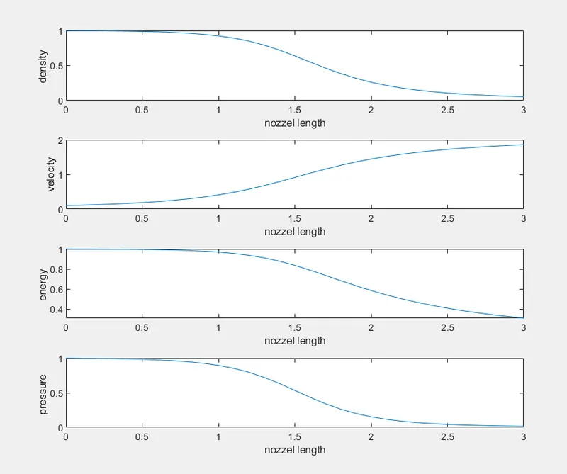
the plot is similar for both Conservative and Non conservative form.
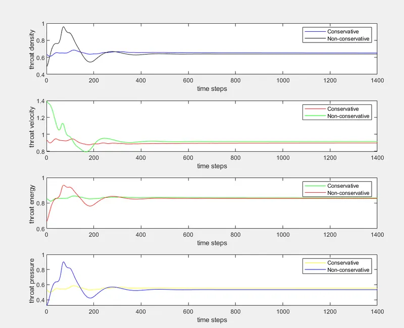
2]Time-wise variation of primitve variables:
3] Variation of Mass flow rate distribution inside the nozzle at different time steps during the time-marching process:
4]Comparison of Normalized mass flow rate distributions of both forms:
Observations:
1] From the first plot we can see the variation of primitive variables along the nozzel length.We know that the nozzel is a Convergent-Divergent nozzel ,with Mach number in convergent region as <1 at throat as =1 and in divergent region as >1. As theory suggests we can observe the velocity increasing along the nozzel length.Also the flow is possible only because of expansion of the gas and hence the decrease in pressure is observed as we predicted.We know that there is a direct relation between pressure and density of a gas.Therfore it can be observed that the density has same behavior as that of the pressure.Eventhough velocity increases, the expansion of the gas causes a decrease in energy .
2]The second plot of primitive varibale at throat Vs the time steps shows that the larger variations are occuring at early times after which the steady state is approached.A wide variation is also seen in the initial time steps because of unsteady expansion and compressive waves formed throught the nozzel in transient.
3] In the third plot we can actually see the convergence of the massflow rate after approximately 750 time steps.In the earlier period it is clearly unsteady.
4]Both conservative and non-conservative methods give a steady solution but conservative method provides better solution since it uses flux variables and not directly the primitive variables.The non-conservative solutions have variations and some oscillations can be seen in both inflow and outflow boundaries.
Grid Dependency Test:
Inorder to understand the grid dependency, we have to change the number of grid points and see if it affects the results.
| Density | Pressure | Temperature | |
| Non-Conservative(n=31) | 0.6387 | 0.5342 | 0.8365 |
| Conservative(n=31) | 0.6524 | 0.5487 | 0.8411 |
| Non-Conservative(n=61) | 0.6377 | 0.5327 | 0.8354 |
| Conservative(n=61) | 0.6390 | 0.5340 | 0.8357 |
Since not much deviation is observed while changing the number of grid points, we can say that our solution is Grid-Independent.
Conclusions:
- Better mass flowrate is obtained in conservative form.
- Ease of programming is in Non-conservative form due to direct interaction with primitive variables unlike Conservative form.
- Steady state is approached quicker in conservative form.
- The solution is grid independent.