Week 3.5 - Deriving 4th order approximation of a 2nd order derivative using Taylor Table method

• Aim: Using Taylor Table Method to derive fourth-order approximation of second-order derivative.
• Theory:

i) The order of accuracy P = Number of nodes in the stencil N - order of derivative Q + 1 for symmetric/central schemes

ii) The order of accuracy P = Number of nodes in the stencil N - order of derivative Q for one-sided/skewed schemes

Skewed-right sided difference can be written as:`frac(del^2u)(delx^2)=frac(af(i)+bf(i+1)+cf(i+2)+df(i+3)+ef(i+4)+gf(i+5))(Deltax^2)`

Taylor's Table for Skewed right sided difference:

`Deltax^2 f''(i)`	`f(i)`	`Deltax f'(i)`	`Deltax^2 f''(i)`	`Deltax^3f'''(i)`	`Deltax^4 f''''(i)`	`Deltax^5f'''''(i)`
`a f(i)`	a	0	0	0	0	0
`b f(i+1)`	`b`	`b`	`frac(b)(2)`	`frac(b)(6)`	`frac(b)(24)`	`frac(b)(120)`
`c f(i+2)`	`c`	`2c`	`frac(4c)(2)`	`frac(8c)(6)`	`frac(16c)(24)`	`frac(32c)(120)`
`d f(i+3)`	`d`	`3d`	`frac(9d)(2)`	`frac(27d)(6)`	`frac(81d)(24)`	`frac(243d)(120)`
`e f(i+4)`	`e`	`4e`	`frac(16e)(2)`	`frac(64e)(6)`	`frac(256e)(24)`	`frac(1024e)(120)`
`g f(+5)`	`g`	`5g`	`frac(25g)(2)`	`frac(125g)(6)`	`frac(625g)(24)`	`frac(3125g)(120)`
	0	0	1	0	0	0

solving the equations vertically we get `a=3.75,b=-12.83333,c=17.83333,d=-13,e=5.08333,g=-0.83333`

Skewed-left sided difference can be written as:`frac(del^2u)(delx^2)=frac(af(i)+bf(i-1)+cf(i-2)+df(i-3)+ef(i-4)+gf(i-5))(Deltax^2)`

Taylor's Table for Skewed left sided difference:

`Deltax^2 f''(i)`	`f(i)`	`Deltax f'(i)`	`Deltax^2 f''(i)`	`Deltax^3f'''(i)`	`Deltax^4 f''''(i)`	`Deltax^5f'''''(i)`
`a f(i)`	a	0	0	0	0	0
`b f(i+1)`	`b`	`-b`	`frac(b)(2)`	`-frac(b)(6)`	`frac(b)(24)`	`-frac(b)(120)`
`c f(i+2)`	`c`	`-2c`	`frac(4c)(2)`	`-frac(8c)(6)`	`frac(16c)(24)`	`-frac(32c)(120)`
`d f(i+3)`	`d`	`-3d`	`frac(9d)(2)`	`-frac(27d)(6)`	`frac(81d)(24)`	`-frac(243d)(120)`
`e f(i+4)`	`e`	`-4e`	`frac(16e)(2)`	`-frac(64e)(6)`	`frac(256e)(24)`	`-frac(1024e)(120)`
`g f(+5)`	`g`	`-5g`	`frac(25g)(2)`	`-frac(125g)(6)`	`frac(625g)(24)`	`-frac(3125g)(120)`
	0	0	1	0	0	0

solving the equations vertically we get `a=3.75,b=-12.83333,c=17.83333,d=-13,e=5.08333,g=-0.83333`

The central difference can be written as :`frac(del^2u)(delx^2)=frac(af(i-2)+bf(i-1)+cf(i)+df(i+1)+ef(i+2))(Deltax^2`

Taylor's Table for Central difference:

`Deltax^2frac(del^2u)(delx^2)`	`f(i)`	`Deltaxf'(i)`	`Deltax^2f''(i)`	`Deltax^3f'''(i)`	`Deltax^4f''''(i)`
`af(i-2)`	`a`	`-2a`	`frac(4a)(2)`	`frac(-8a)(6)`	`frac(16a)(24)`
`bf(i-1)`	`b`	`-b`	`fracb2`	`frac(-b)6`	`frac(b)(24)`
`cf(i)`	`c`	`0`	`0`	`0`	`0`
`df(i+1)`	`d`	`d`	`fracd2`	`fracd6`	`frac(d)(24)`
`ef(i+2)`	`e`	`2e`	`frac(4e)(2)`	`frac(8e)(6)`	`frac(16e)(24)`
	0	0	1	0	0

Solving for the equations vertically we get`a=-0.08333,b=1.33333,c=-2.5,d=1.333333,e=-0.08333`

• Sample Code:

close all
clear all
clc
%skewed_right_sided_diff=((3.75*f(x))-(12.8333*f(x+dx))+(17.8333*f(x+2*dx))-(13*f(x+3*dx))+(5.0833*f(x+4*dx))-(0.8333*f(x+5*dx)))/dx^2
%skewed_left_sided_diff=((3.75*f(x))-(12.8333*f(x+dx))+(17.8333*f(x+2*dx))-(13*f(x+3*dx))+(5.0833*f(x+4*dx))-(0.8333*f(x+5*dx)))/dx^2
%central_diff=((-0.08333*f(x-2*dx))+(1.3333*f(x-dx))-(2.5*f(x))+(1.3333*f(x+dx))-(0.8333*f(x+2*dx)))/dx^2

%function to examine is e^x .cos(x)
%  exact second derivative of given function is -2*e^x sin(x)
x=pi/3;
%dx=(pi/4000 : 0.0019 : pi/40);
dx = linspace(pi/4000,pi/40,40);
exact_diff= -2*exp(x)*sin(x);
for i=1:length(dx)
    
    central_diff(i)=(-( 0.083333333333333333333333333333333333*exp(x-(2*dx(i)))*cos(x-(2*dx(i)))) + (1.3333333333333333333333333333333333333*(exp(x-dx(i))*cos(x-dx(i)))) - (2.5*(exp(x)*cos(x))) + (1.3333333333333333333333333333333333333*(exp(x+dx(i))*cos(x+dx(i)))) - (0.08333333333333333333333333333333333333*(exp(x+(2*dx(i)))*cos(x+(2*dx(i))))))/(dx(i)^2);
    
    skewed_right_sided_diff(i)=((3.75*(exp(x)*cos(x))) - (12.83333333333333333333333333333333333*(exp(x+dx(i))*cos(x+dx(i)))) + (17.8333333333333333333333333333333333333*(exp(x+(2*dx(i)))*cos(x+(2*dx(i))))) - (13*(exp(x+(3*dx(i)))*cos(x+(3*dx(i))))) + (5.0833333333333333333333333333333333333*(exp(x+(4*dx(i)))*cos(x+(4*dx(i))))) - (0.833333333333333333333333333333333333*(exp(x+(5*dx(i)))*cos(x+(5*dx(i))))))/(dx(i)^2);
    
    skewed_left_sided_diff(i)=((3.75*(exp(x)*cos(x))) - (12.83333333333333333333333333333333333*(exp(x-dx(i))*cos(x-dx(i)))) + (17.83333333333333333333333333333333333333*(exp(x-(2*dx(i)))*cos(x-(2*dx(i)))))-(13*(exp(x-(3*dx(i)))*cos(x-(3*dx(i)))))+(5.08333333333333333333333333333333333*(exp(x-(4*dx(i)))*cos(x-(4*dx(i)))))-(0.8333333333333333333333333333333333333*(exp(x-(5*dx(i)))*cos(x-(5*dx(i))))))/(dx(i)^2);
    
    error_central(i)=abs(central_diff(i)-exact_diff);
    error_skew_right(i)=abs(skewed_right_sided_diff(i)-exact_diff);
    error_skew_left(i)=abs(skewed_left_sided_diff(i)-exact_diff);
    
end
%plot(dx,error_central,'color','blue');hold on;
%plot(dx,error_skew_right,'color','red');hold on;
%plot(dx,error_skew_left,'color','green');
loglog(dx,error_central,'color','blue');hold on;
loglog(dx,error_skew_right,'color','red');hold on;
loglog(dx,error_skew_left,'color','green');
legend('central error','skewed right sided error','skewed left sided error');
xlabel('range of dx');
ylabel('error');

• Understanding the code: The code is simply a for loop running for each element in the dx array. The mathematical equation for each approximation is calculated using Taylor's table method and the coefficient of each approximation is calculated through matrix representation of the system of equations. An exact derivative is calculated using the product rule of differentiation. The absolute difference is calculated using the function available in Matlab as 'abs()'.The plot of error of each approximation Vs the dx range is plotted to analyze.
• Plot:

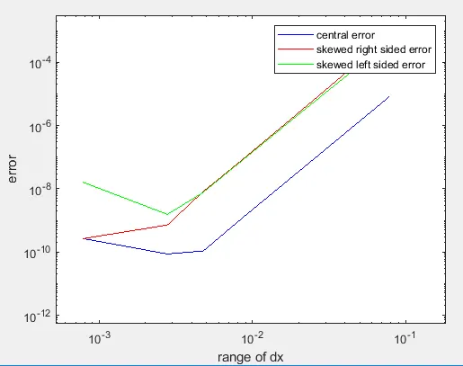
• Variance in the plot: Variations in the plot are observed when the round-off terms are limited. This is because at smaller ranges of dx the approximation errors are varied due to truncated terms in the approximated terms. If after the decimal the number of terms is limited to 5 then we get a different plot than we get if it is limited to 10 or 15 and so on.
• Result and Discussion: We can see that the central difference gives the least error compared to the skewed right or skewed left differences. But the advantage that skewed side differences hold compared to central differences is that at domains where starting stencil has to be approximated and no stencils are available before it or after it we will have to go along with skewed right or skewed left as required. But Central differences since it consists of information from both sides would yield betters results.