Week 11 - Simulation of Flow through a pipe in OpenFoam
Aim: To simulate an axi-symmetric flow by applying the wedge boundary condition.The flow is laminar and flows through a constant cross-section pipe at an inlet Reynold's number of 2100.
- Validate Hydro-dynamic length with the numerical result
- Validate the fully developed flow velocity profile with its analytical profile
- Validate maximum velocity and pressured drop for fully developed flow
- Post-process Shear stress and validate wall shear stress for fully developed flow
Theory: Hagen-Poiseuille's law is the law which governs the pressure drop in a laminar flow of incompressible newtonian fluis in a long cylindrical pipe.Consider a fluid enterning a pipe.Due to no slip conditions the fluid particles closer to the pipe surface are going to stick to the surface and loose their velocity to zero.As a result the fluid layer just above it will feel the drag caused by the bottom layer .This is known as the viscous drag.As a result the velocity of the fluid layers decreases from the free stream velocity.Inorder to maintian constant mass flow rate , the free stream which is away from the effect of the viscous drag will have to increase its velocity.Hence there occurs a velocity gradient in the region. The region in which th eviscous drag can be felt is called as the BOUNDARY LAYER.
This boundary layer divides the flow into two regimes , one is the one in which the viscous effects can be seen and the other is where the free stream exists.The thickness of the boundary layer is going to increase in the direction of the flow unless it reaches the centre of the pipeline.The region of the pipe line from inlet to the the point where the boundary layer merges together at the pipe centreline is called the HYDRODYNAMIC ENTRANCE REGION and the length is called as HYDRODYNAMIC ENTRANCE LENGTH.
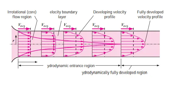
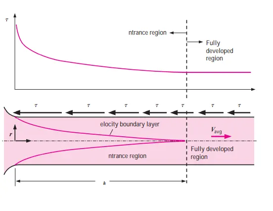
The above figure shows the boundary layer formations and its merging towards the centreline.
Since it is going to be computationally heavy to simulate the flow over the whole of pipe, we are going to consider only a wedge with angle 5degree, and then reflect the properties over the diameter to resembel the pipe flow.
Operating Conditions:
Reynold's Number:It is a non dimensional number which compares the effects of vicous and inertia force.It is given as ration of inertia force to viscous force.`Re=(rho*v*d)/mu`
Here we are given to examine the flow under laminar co`10^(-6)`nditions with a Reynold's number as 2100. With the above equation we have to find the inlet velocity to be given to the flow.
Hydrodynamic Entry Length: Since the flow is laminar , the equation goes as `Le=0.06*d*Re`
Velocity Profile:
`V(r)=V_(max) * (1- r^2 /R^2 )`
`V_(max) =2* V_(avg)`
Pressure Drop: It gives the difference in pressure between two points in the pipe along the flow.
The Hagen-Poiseuille's equation for the presure drop is given as `Deltap =(32 * mu*V*L )/d^2`
Assumptions and variables:
Pipe dia:0.03m
fluid:water
density of wawter=997`(kg)/m^3`
dynamic viscosity of water=0.001 `Pa.s`
kinematic viscsity of water=1.003*`10^(-6)``m^2 /s`
Hydrodynamic entry length=3.78m
V_avg=0.072m/s
v_max=0.1404m/s
Matlab Code for blockmesh:
close all
clear all
clc
%creating blockmeshdict for openfoam
Re=2100;%Reynold's Number
D=input('dia of pipe :');% Diameter of pipe
r=D/2;%radius of the pipe
Le=0.06*Re*D;%entry length of pipe
L=Le+1;%total length of pipe
mu=0.001;%Dynamic viscosityt of water
rho=997;%density of water


%wedge angle
theta=input('inputwedge angle :');

%simple grading
nx=200;
ny=21;
nz=1;


%average velocity of flow in pipe
v_avg= (mu*Re)/(rho*D);
%max velocity of flow in pipe
v_max=2*v_avg;

%pressure drop
delta_p= (32*mu*v_avg*L)/(D^2);
 t=L/v_avg;


%CREATING BLOCKMESH FILE

h1='/*--------------------------------*- C++ -*----------------------------------*\';
h2='  =========                 |';
h3='  \\      /  F ield         | OpenFOAM: The Open Source CFD Toolbox';
h4='   \\    /   O peration     | Website:  https://openfoam.org';
h5='    \\  /    A nd           | Version:  9';
h6='     \\/     M anipulation  |';
h7='\*---------------------------------------------------------------------------*/';
h8='FoamFile';
h9='{';
h10='    format      ascii;';
h11='    class       dictionary;';
h12='    object      blockMeshDict;';
h13='}';
h14='// * * * * * * * * * * * * * * * * * * * * * * * * * * * * * * * * * * * * * //';
h15='// ************************************************************************* //';


%OPENING A FILE

f1=fopen('blockMeshDict.txt','w');

%writing header comments
fprintf(f1,'%s\n',h1);
fprintf(f1,'%s\n',h2);
fprintf(f1,'%s\n',h3);
fprintf(f1,'%s\n',h4);
fprintf(f1,'%s\n',h5);
fprintf(f1,'%s\n',h6);
fprintf(f1,'%s\n',h7);
fprintf(f1,'%s\n',h8);
fprintf(f1,'%s\n',h9);
fprintf(f1,'%s\n',h10);
fprintf(f1,'%s\n',h11);
fprintf(f1,'%s\n',h12);
fprintf(f1,'%s\n',h13);
fprintf(f1,'%s\n',h14);
%vertices
fprintf(f1,'convertToMeters 1 \n');
fprintf(f1,'vertices \n');
fprintf(f1,'( \n');
fprintf(f1,'%d %d %d\n',0,0,0);
fprintf(f1,'%d %d %d\n',0,r*cosd(theta/2),r*sind(theta/2));
fprintf(f1,'%d %d %d\n',0,r*cosd(theta/2),-r*sind(theta/2));
fprintf(f1,'%d %d %d\n',L,0,0);
fprintf(f1,'%d %d %d\n',L,r*cosd(theta/2),r*sind(theta/2));
fprintf(f1,'%d %d %d\n',L,r*cosd(theta/2),-r*sind(theta/2));
fprintf(f1,'); \n');

%creating blocks
fprintf(f1,'blocks \n');
fprintf(f1,'( \n');
fprintf(f1,'hex (0 3 5 2 0 3 4 1)(%d %d %d) simpleGrading(1 0.2 1) \n',nx,ny,nz);
fprintf(f1,'); \n');

%creating edges
fprintf(f1,'edges \n');
fprintf(f1,'( \n');
fprintf(f1,'arc 1 2 (0 %d 0) \n' ,r);
fprintf(f1,'arc 4 5 (%d %d 0) \n' ,L,r);
fprintf(f1,'); \n');


%specifying boundary
fprintf(f1,'boundary \n');
fprintf(f1,'( \n');
%axis
fprintf(f1,'\t axis \n');
fprintf(f1,'\t{ \n');
fprintf(f1,'\t type empty ;\n');
fprintf(f1,'\t faces \n');
fprintf(f1,'\t\t( \n');
fprintf(f1,'\t\t (0 3 3 0) \n');
fprintf(f1,'\t\t); \n');
fprintf(f1,'\t} \n');

%wall
fprintf(f1,'\t wall \n');
fprintf(f1,'\t{ \n');
fprintf(f1,'\t type wall ;\n');
fprintf(f1,'\t faces \n');
fprintf(f1,'\t\t( \n');
fprintf(f1,'\t\t (1 4 5 2) \n');
fprintf(f1,'\t\t); \n');
fprintf(f1,'\t} \n');


%inlet
fprintf(f1,'\t inlet \n');
fprintf(f1,'\t{ \n');
fprintf(f1,'\t type patch ;\n');
fprintf(f1,'\t faces \n');
fprintf(f1,'\t\t( \n');
fprintf(f1,'\t\t (0 1 2 0) \n');
fprintf(f1,'\t\t); \n');
fprintf(f1,'\t} \n');

%outlet
fprintf(f1,'\t outlet \n');
fprintf(f1,'\t{ \n');
fprintf(f1,'\t type patch ;\n');
fprintf(f1,'\t faces \n');
fprintf(f1,'\t\t( \n');
fprintf(f1,'\t\t (3 5 4 3) \n');
fprintf(f1,'\t\t); \n');
fprintf(f1,'\t} \n');


%front
fprintf(f1,'\t front \n');
fprintf(f1,'\t{ \n');
fprintf(f1,'\t type wedge ;\n');
fprintf(f1,'\t faces \n');
fprintf(f1,'\t\t( \n');
fprintf(f1,'\t\t (0 3 4 1) \n');
fprintf(f1,'\t\t); \n');
fprintf(f1,'\t} \n');


%back
fprintf(f1,'\t back \n');
fprintf(f1,'\t{ \n');
fprintf(f1,'\t type wedge ;\n');
fprintf(f1,'\t faces \n');
fprintf(f1,'\t\t( \n');
fprintf(f1,'\t\t (0 2 5 3) \n');
fprintf(f1,'\t\t); \n');
fprintf(f1,'\t} \n');

fprintf(f1,'); \n');

fprintf(f1,'mergePatchPairs \n');
fprintf(f1,'( \n');
fprintf(f1,'); \n');

fprintf(f1,'%s\n',h15);
Procedure:
- After opening the terminal ,we need to choose the relevant tutorial file and copy it to the RUN folder and excecute the changes there.
- change the blockMeshDict file with the one we created using Matlab code.The blockmesh file will look as shown.
blockMeshDict
/*--------------------------------*- C++ -*----------------------------------*\
  =========                 |
  \\      /  F ield         | OpenFOAM: The Open Source CFD Toolbox
   \\    /   O peration     | Website:  https://openfoam.org
    \\  /    A nd           | Version:  9
     \\/     M anipulation  |
\*---------------------------------------------------------------------------*/
FoamFile
{
    format      ascii;
    class       dictionary;
    object      blockMeshDict;
}
// * * * * * * * * * * * * * * * * * * * * * * * * * * * * * * * * * * * * * //
convertToMeters 1 ;

vertices
(
 (0 0 0)
 (0 1.498572e-02 6.542908e-04)
 (0 1.498572e-02 -6.542908e-04)
 (4.780000e+00 0 0)
 (4.780000e+00 1.498572e-02 6.542908e-04)
 (4.780000e+00 1.498572e-02 -6.542908e-04)
);

blocks
(
hex (0 3 5 2 0 3 4 1) (200 21 1) simpleGrading (1 0.2 1)
);

edges
(
arc 1 2 (0 1.500000e-02 0)
arc 4 5 (4.780000e+00 1.500000e-02 0)
);

boundary
(
	 axis
	{
	 type empty ;
	 faces
		(
		 (0 3 3 0)
		);
	}

	 wall
	{
	 type wall ;
	 faces
		(
		 (1 4 5 2)
		);
	}

	 inlet
	{
	 type patch ;
	 faces
		(
		 (0 1 2 0)
		);
	}

	 outlet
	{
	 type patch ;
	 faces
		(
		 (3 5 4 3)
		);
	}

	 front
	{
	 type wedge ;
	 faces
		(
		 (0 3 4 1)
		);
	}

	 back
	{
	 type wedge ;
	 faces
		(
		 (0 2 5 3)
		);
	}
);
mergePatchPairs
(
);
// ************************************************************************* //
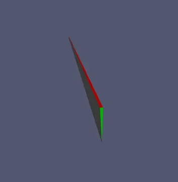
The wedge looks as shown below:
- After this we edit the ControlDict file to set up the time steps inorder to achieve a stable solution with CFL<1.
controlDict
/*--------------------------------*- C++ -*----------------------------------*\
  =========                 |
  \\      /  F ield         | OpenFOAM: The Open Source CFD Toolbox
   \\    /   O peration     | Website:  https://openfoam.org
    \\  /    A nd           | Version:  9
     \\/     M anipulation  |
\*---------------------------------------------------------------------------*/
FoamFile
{
    format      ascii;
    class       dictionary;
    location    "system";
    object      controlDict;
}
// * * * * * * * * * * * * * * * * * * * * * * * * * * * * * * * * * * * * * //

application     icoFoam;

startFrom       startTime;

startTime       0;

stopAt          endTime;

endTime         70;

deltaT          0.01;

writeControl    timeStep;

writeInterval   20;

purgeWrite      0;

writeFormat     ascii;

writePrecision  6;

writeCompression off;

timeFormat      general;

timePrecision   6;

runTimeModifiable true;


// ************************************************************************* //
- We have to set up the inlet conditons for velocity as well as pressure.The inlet value of velocity is the one we had calculated using the reynold's formula.Pressure value at inlet is to be maintained as the one as atmospheric.Hence the gauge becomes zero.THe conditions for both velocity and pressure is to be intialised as uniform.
Velocity
/*--------------------------------*- C++ -*----------------------------------*\
========= |
\\ / F ield | OpenFOAM: The Open Source CFD Toolbox
\\ / O peration | Website: https://openfoam.org
\\ / A nd | Version: 9
\\/ M anipulation |
\*---------------------------------------------------------------------------*/
FoamFile
{
format ascii;
class volVectorField;
object U;
}
// * * * * * * * * * * * * * * * * * * * * * * * * * * * * * * * * * * * * * //
dimensions [0 1 -1 0 0 0 0];
internalField uniform (0 0 0);
boundaryField
{
inlet
{
type fixedValue;
value uniform (0.072 0 0);
}
outlet
{
type zeroGradient;
}
wall
{
type noSlip;
}
axis
{
type empty;
}
front
{
type wedge;
}
back
{
type wedge;
}
}
// ************************************************************************* //
Pressure
/*--------------------------------*- C++ -*----------------------------------*\
  =========                 |
  \\      /  F ield         | OpenFOAM: The Open Source CFD Toolbox
   \\    /   O peration     | Website:  https://openfoam.org
    \\  /    A nd           | Version:  9
     \\/     M anipulation  |
\*---------------------------------------------------------------------------*/
FoamFile
{
    format      ascii;
    class       volScalarField;
    object      p;
}
// * * * * * * * * * * * * * * * * * * * * * * * * * * * * * * * * * * * * * //

dimensions      [0 2 -2 0 0 0 0];

internalField   uniform 0;

boundaryField
{
    inlet
    {
        type            zeroGradient;
    }

    outlet
    {
        type            fixedValue;
        value uniform 0;
    }


    wall
    {
        type            zeroGradient;
    }

    front
    {
        type            wedge;
    }

    back
    {
        type            wedge;
    }
}

// ************************************************************************* //
- The transport ptoperties script inside the constant folder should be taken care of since it has the most important property i.e the kinmatic viscosity.
transportProperties
/*--------------------------------*- C++ -*----------------------------------*\
  =========                 |
  \\      /  F ield         | OpenFOAM: The Open Source CFD Toolbox
   \\    /   O peration     | Website:  https://openfoam.org
    \\  /    A nd           | Version:  9
     \\/     M anipulation  |
\*---------------------------------------------------------------------------*/
FoamFile
{
    format      ascii;
    class       dictionary;
    location    "constant";
    object      transportProperties;
}
// * * * * * * * * * * * * * * * * * * * * * * * * * * * * * * * * * * * * * //

nu              [0 2 -1 0 0 0 0] 0.000001003;


// ************************************************************************* //
Results and Observations:
- formation of fully developed velocity profile:
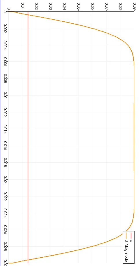
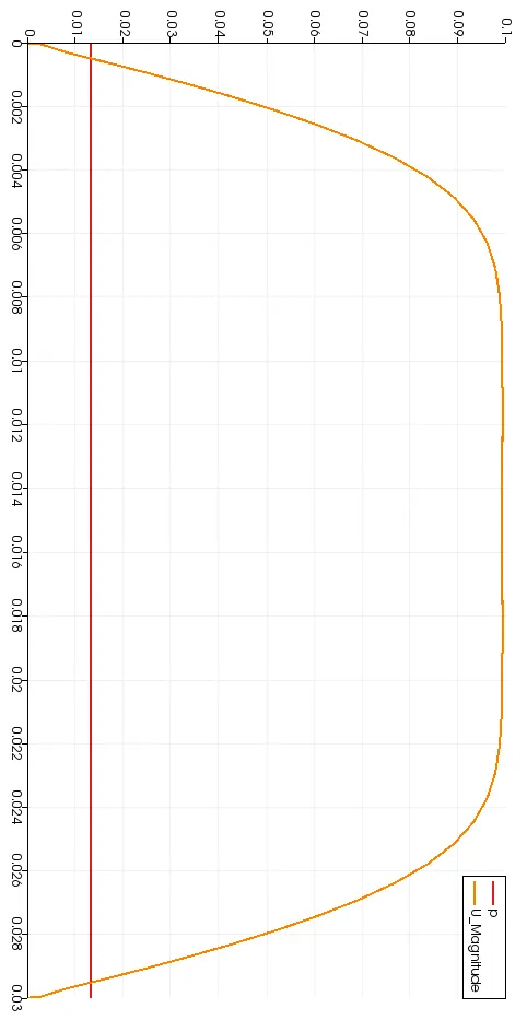
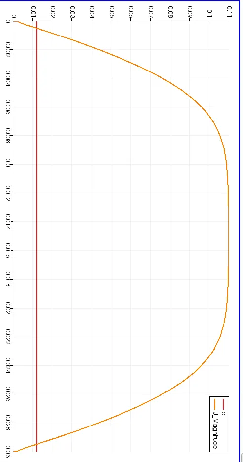
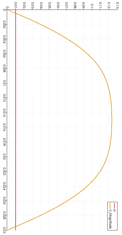
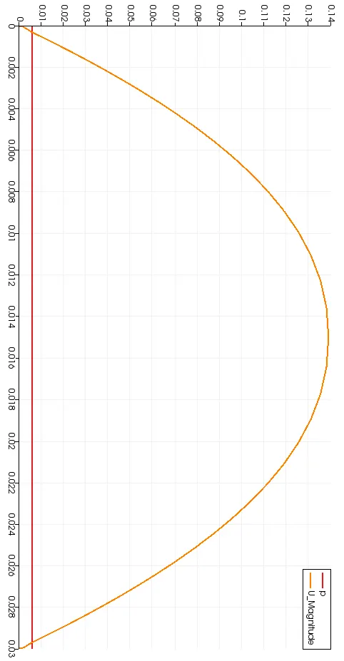
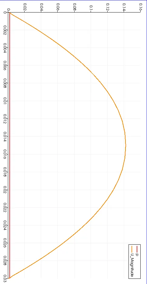
The above velocity profiles are found at distances of 0.1m,0.25m,0.5m,1.2m,2.5m and 4m from the inlet of the pipe.
From Hagen-Poisuellie's law we had derived the velocity profile of the fluid inside the boundary layer as parabolic , which is observed as above.Also after the entry length the velocity profile is not changing since the slow is fully developed.
- Centerline velocity over the length of the pipe:
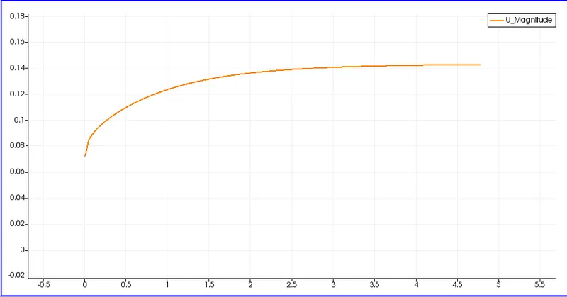
It can be clearly seen that the velocity is increasing .This is explained by the conservation of mass.Since we are plotting the centreline velocity, and the formation of boundarylayer is going to reduce the massflowrate due to decrease in velocity inside the boundary layer, the free stream velocity is going to increase inorder to maintain the mass flow rate.Also after the analytical hydodynamic entry legth there is no much drastic change in the velocity since there exists fully developed flow.
- Centerline pressure over length of pipe
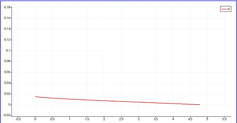
From Bernoulli's principle we do know that the total energy head has to remain constant and since there is no change in the potential head, with increase in velocity pressure should be decreasisng.But inorder to maintain the flow the pressure decreases further after the entry length.This can also considered as the decreases in energy due to frictional losses.
- calculating shear stress:
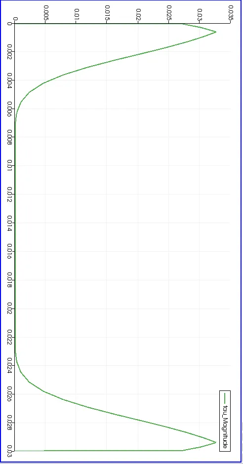
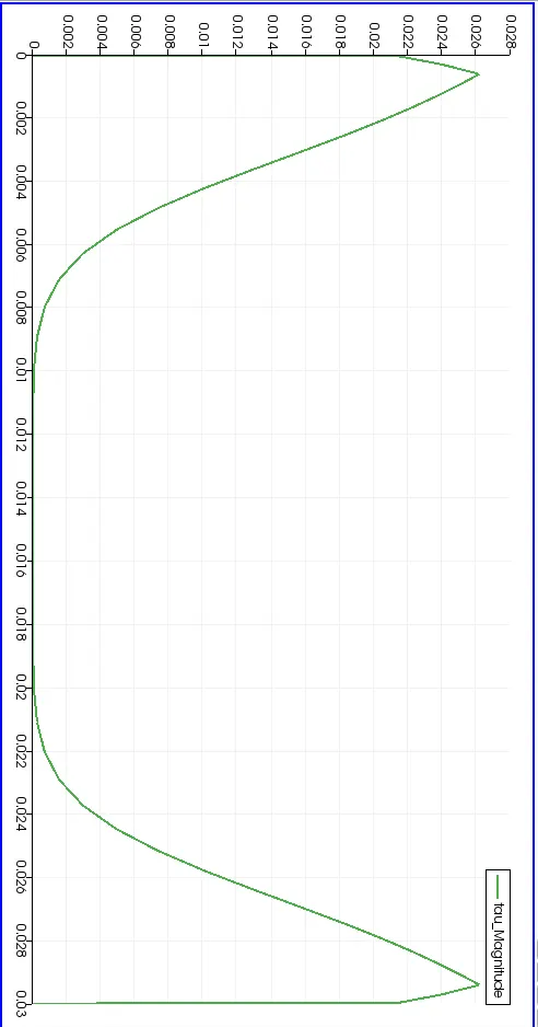
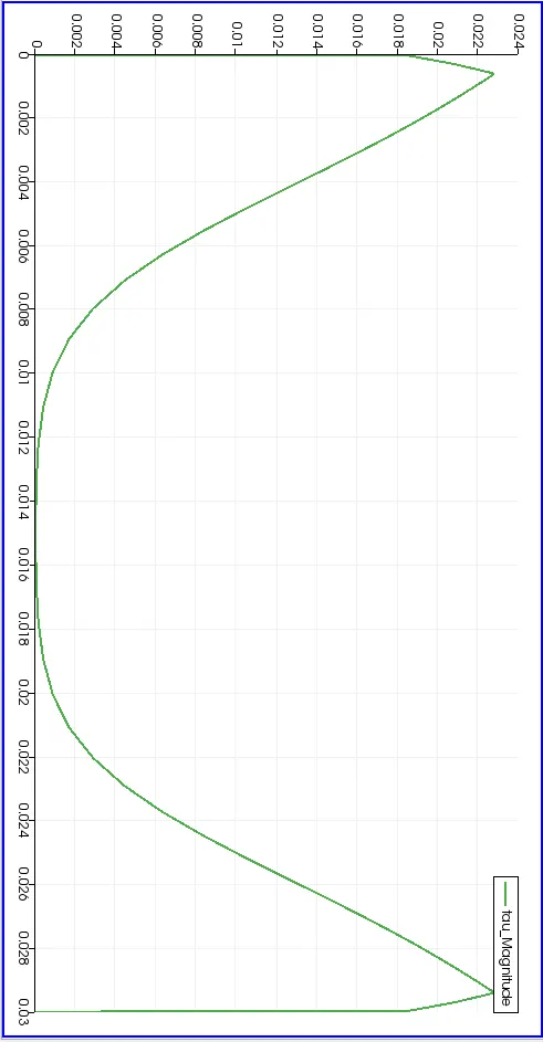
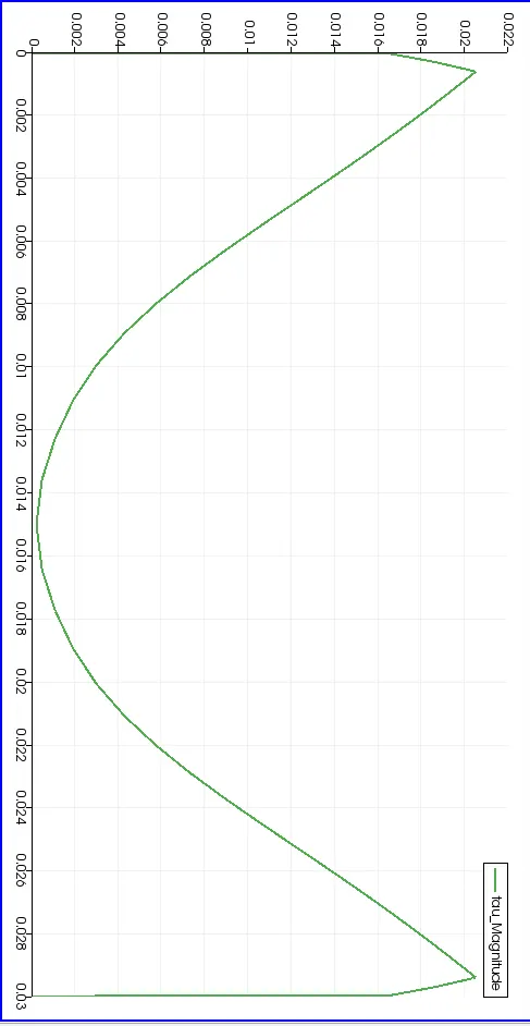
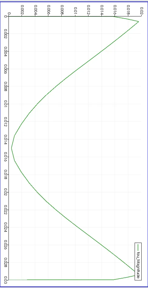
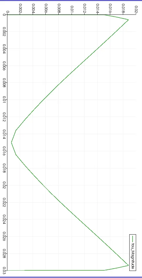
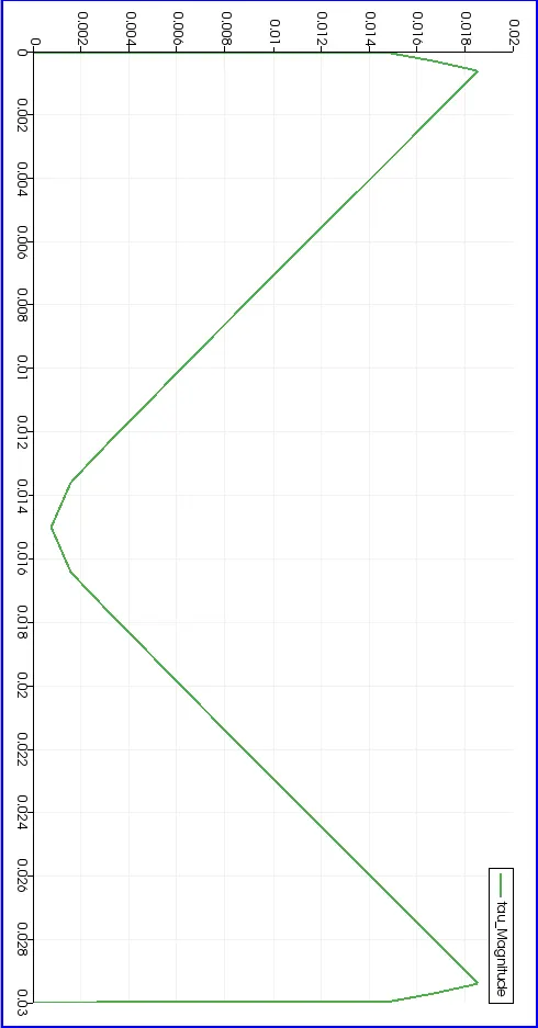
The above plots shows how the shear stress varies across the cross section from the start of the pipe towards its end. Plots are representing the distance of 0.1m,0.25m,0.5m,1m,1.5m,2.5mand 4m from the entrance of the pipe.
It can be clearly seen that the variation of shear stress is linear as we observe from the newtonian equation `tau=mu* (delu )/(dely)` .
The shear stress is zero at the centre line of the pipe.Lets see an interesting plot here.
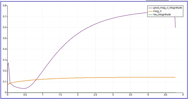
The above plot shows the variation of magnitude of velocity shear stress and the gradient of velocity. We know that the shear stressis zero along the centerline.But dynamic viscosity cannot be zero then how is it possible? Either the gradient should be zero or there is something we are missing.
Clearly the gradient is not zero in the centerline since inorder to maintain the mass flow rate the velocity not only ncreases but also there is some mixing taking place.As far as shear stress is concerned ,shear stress is predominant only closer to a solid boundary.
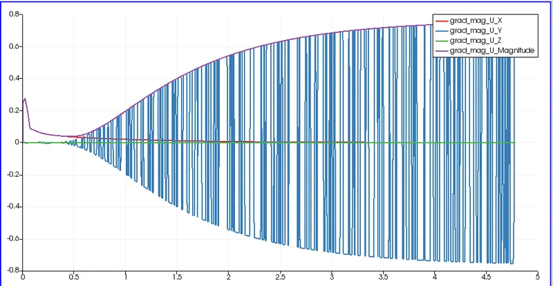
As we know the gradient to a scalar is a vector ,we can see the variation in each direction of the velocity. The presence of mixing can be proved here with the presence of gradients in x and y though it is in free stream .
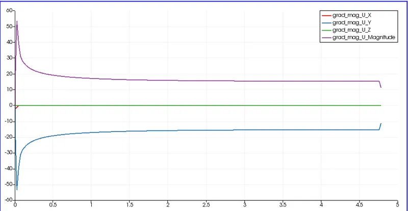
In the above graph the plot is made closer to the wall and we can see the presence of shear stress and gradient only in y direction.
Our use of reflecting properties will show some anomalities , but the inference will be the same as we expect.